F: Estudio de isofotas
Una isofota se define como:
«Una línea que une puntos con el mismo brillo superficial en un diagrama o una imagen de un objeto celeste como una galaxia o una nebulosa.»
El brillo superficial \(\mu\) (mu) generalmente se mide en magnitudes por segundo de arco al cuadrado. La suma de toda la luz dentro de una isofota dada se denomina magnitud isofotal.
Si el perfil luminoso de una galaxia es elíptico, sus isofotas serán elipses.
El paquete isophote proporciona herramientas para ajustar isófotas elípticas a una imagen de una galaxia. Las isófotas de la imagen se miden usando un método iterativo descrito por Jedrzejewski (1987; MNRAS 226, 747).
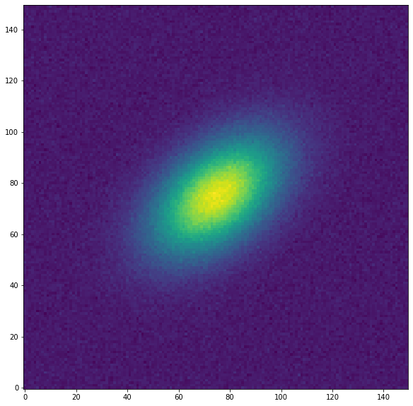
Para este ejemplo, vamos a crear una imagen de galaxia simulada simple:
[1]:
from astropy.modeling.models import Gaussian2D
import numpy as np
from photutils.datasets import make_noise_image
import matplotlib.pyplot as plt
[2]:
g = Gaussian2D(100., 75, 75, 20, 12, theta=40. * np.pi / 180.) # generamos una gausiana eliptica en 2d girada 40 grados
ny = nx = 150 #cantidad de pixeles en x e y
y, x = np.mgrid[0:ny, 0:nx]
noise = make_noise_image((ny, nx), distribution='gaussian', mean=0., # metemos algo de ruido
                         stddev=2., seed=1234)
data = g(x, y) + noise
[3]:
plt.figure("Galaxia", figsize=[10, 10])
plt.imshow(data, origin='lower')
plt.show()
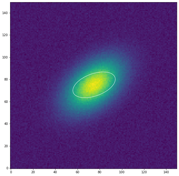
Debemos proporcionar una elipse al ajuste de las isófotas como condición inicial. Esta geometría de la elipse se define con la clase EllipseGeometry. Aquí definiremos una elipse inicial cuyo ángulo de posición está desplazado respecto los datos.
[4]:
from photutils.isophote import EllipseGeometry
geometry = EllipseGeometry(x0=75, y0=75, sma=20, eps=0.5,
                           pa=20. * np.pi / 180.)
Vamos a mostrar esta elipse inicial:
[5]:
from photutils.aperture import EllipticalAperture
aper = EllipticalAperture((geometry.x0, geometry.y0), geometry.sma,
                          geometry.sma * (1 - geometry.eps),
                          geometry.pa)
plt.figure("Galaxia", figsize=[10, 10])
plt.imshow(data, origin='lower')
aper.plot(color='white')
plt.show()
A continuación, creamos una instancia de la clase Ellipse, donde tendremos en cuenta los datos que se ajustarán, es decir la imagen de la galaxia y la elipse inicial:
[6]:
from photutils.isophote import Ellipse
ellipse = Ellipse(data, geometry)
Para realizar el ajuste de isófotas elípticas, ejecutamos el método fit_image() :
[7]:
isolist = ellipse.fit_image()
El resultado es una lista de isófotas, cuyos atributos son los valores del ajuste para cada una de las isofotas ordenadas por la longitud del semieje mayor. Veamos los ángulos de posición de ajuste (en radianes):
[8]:
isolist.pa
[8]:
array([0.00000000e+00, 2.58557691e-02, 1.24258032e-02, 2.81651474e-03,
       3.10564077e+00, 3.01432668e+00, 2.91207413e+00, 2.55353790e+00,
       3.27667134e-01, 3.12991751e+00, 3.12991751e+00, 1.60073797e-02,
       3.13170982e+00, 8.28190557e-02, 1.04356317e-01, 1.58706115e-01,
       3.20421940e-01, 3.82976829e-01, 4.85453395e-01, 7.06300855e-01,
       1.14601352e+00, 1.00547579e+00, 9.73052854e-01, 6.24088491e-01,
       5.79963706e-01, 6.24163539e-01, 7.36384503e-01, 7.64785040e-01,
       6.98341037e-01, 6.77667042e-01, 6.81952942e-01, 6.27394019e-01,
       6.64901758e-01, 6.91061656e-01, 6.96059953e-01, 6.93651837e-01,
       6.86072223e-01, 6.78834001e-01, 6.91164283e-01, 7.06300855e-01,
       6.87382951e-01, 6.78429447e-01, 6.91862441e-01, 6.88541138e-01,
       6.89746530e-01, 7.04616954e-01, 6.98198654e-01, 7.02949641e-01,
       6.87174406e-01, 6.87174406e-01, 6.87174406e-01, 7.36770379e-01,
       7.36770379e-01, 7.36770379e-01])
También podemos mostrar los valores de las isófotas como una tabla, que nuevamente se ordena por la longitud del semieje mayor (sma):
[9]:
print(isolist.to_table())
       sma               intens            intens_err      ... niter stop_code
                                                           ...
------------------ ------------------ -------------------- ... ----- ---------
               0.0  103.3660741932861                  0.0 ...     0         0
0.5346972612827552 101.85768930454661 0.030160181107668268 ...    10         0
0.5881669874110307 101.68151143393658 0.028309622593685645 ...    10         0
0.6469836861521338   101.505670787118 0.025866912481304023 ...    11         0
0.7116820547673471   101.372109520222  0.03225393307834451 ...    10         0
0.7828502602440819 101.18631230115908   0.0361583334561795 ...    10         0
0.8611352862684901 100.96908841886025  0.03258843615160212 ...    10         0
0.9472488148953392 100.78891350007841 0.049768537796437626 ...    10         0
1.0419736963848731 100.42647733875044  0.08087063557978552 ...    19         0
1.1461710660233606  100.2813456048825  0.08525970834625504 ...    50         2
               ...                ...                  ... ...   ...       ...
 32.21020000000001  27.26171456357163  0.10957850079687152 ...    10         0
 35.43122000000001 20.802860058616794  0.09299435657992926 ...    10         0
38.974342000000014 15.038704467533424  0.09788537700939103 ...    10         0
 42.87177620000002  9.957840971954045  0.09606873371025618 ...    10         0
 47.15895382000003  6.094966160355057  0.08299661880443569 ...    10         0
51.874849202000036 3.4153177276271887  0.07834803763518963 ...    10         0
 57.06233412220004 1.5518907342094141  0.08731774884195193 ...    50         2
 62.76856753442005 0.7074698044512818  0.07602993679767285 ...    50         2
 69.04542428786206  0.250073095540471  0.06955238583559703 ...     3         5
 75.94996671664828 0.1403359017804461  0.07032595343951609 ...     2         5
Length = 54 rows
[10]:
fig, (ax1) = plt.subplots(figsize=(14, 5), nrows=1, ncols=1)
fig.subplots_adjust(left=0.04, right=0.98, bottom=0.02, top=0.98)
ax1.imshow(data, origin='lower')
ax1.set_title('Ajuste de isofotas')

smas = np.linspace(10, 50, 10) # definimos ciertos valores de sma
for sma in smas:
    iso = isolist.get_closest(sma) # vemos las isofotas que estan mas cerca de los sma definidas
    x, y, = iso.sampled_coordinates()
    ax1.plot(x, y, color='white')
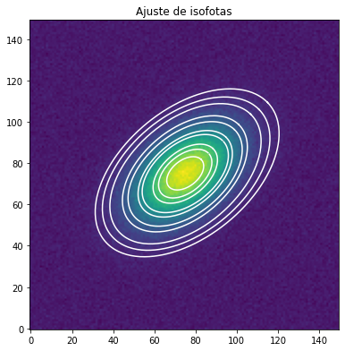
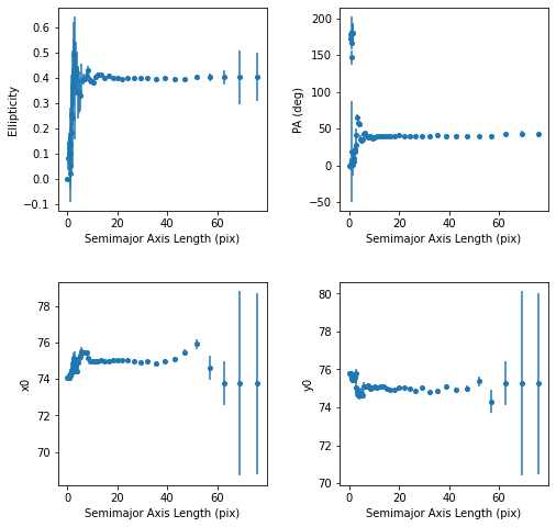
Vemos varios parámetros de del ajuste de las isofotas
[11]:
plt.figure(figsize=(8, 8))
plt.subplots_adjust(hspace=0.35, wspace=0.35)

plt.subplot(2, 2, 1)
plt.errorbar(isolist.sma, isolist.eps, yerr=isolist.ellip_err,
             fmt='o', markersize=4)
plt.xlabel('Semimajor Axis Length (pix)')
plt.ylabel('Ellipticity')

plt.subplot(2, 2, 2)
plt.errorbar(isolist.sma, isolist.pa / np.pi * 180.,
             yerr=isolist.pa_err / np.pi * 80., fmt='o', markersize=4)
plt.xlabel('Semimajor Axis Length (pix)')
plt.ylabel('PA (deg)')

plt.subplot(2, 2, 3)
plt.errorbar(isolist.sma, isolist.x0, yerr=isolist.x0_err, fmt='o',
             markersize=4)
plt.xlabel('Semimajor Axis Length (pix)')
plt.ylabel('x0')

plt.subplot(2, 2, 4)
plt.errorbar(isolist.sma, isolist.y0, yerr=isolist.y0_err, fmt='o',
             markersize=4)
plt.xlabel('Semimajor Axis Length (pix)')
plt.ylabel('y0')
plt.show()
Podemos construir una imagen modelo a partir del objeto IsophoteList usando la funcion build_ellipse_model():
[12]:
from photutils.isophote import build_ellipse_model
model_image = build_ellipse_model(data.shape, isolist)
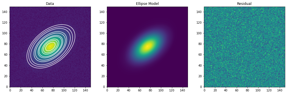
Finalmente, graficamos los datos originales, superpuestos con algunas de las isófotas, la imagen del modelo elíptico y la imagen residual:
[13]:
residual = data - model_image

fig, (ax1, ax2, ax3) = plt.subplots(figsize=(14, 5), nrows=1, ncols=3)
fig.subplots_adjust(left=0.04, right=0.98, bottom=0.02, top=0.98)
ax1.imshow(data, origin='lower')
ax1.set_title('Data')

smas = np.linspace(10, 50, 10)
for sma in smas:
    iso = isolist.get_closest(sma)
    x, y, = iso.sampled_coordinates()
    ax1.plot(x, y, color='white')

ax2.imshow(model_image, origin='lower')
ax2.set_title('Ellipse Model')

ax3.imshow(residual, origin='lower')
ax3.set_title('Residual')
[13]:
Text(0.5, 1.0, 'Residual')
Ejemplo de isofotas M51
Usaremos un ejemplo real de la galaxia M51. Tenemos que tener en cuenta que M51, con sus brazos espirales y regiones HII, no es la mejor galaxia para el análisis por el algoritmo de “ellipse”, ya que asume que las isófotas son principalmente de forma elíptica. Por otro lado, la imagen M51 es ideal para comprobar la eficiencia del algoritmo frente a la contaminación de la imagen por características no elípticas.
Vamos a leer nuestra imagen desde una URL
[14]:
from astropy.io import fits
from astropy.utils.data import download_file

url = 'https://github.com/astropy/photutils-datasets/raw/main/data/isophote/M51.fits'
path = download_file(url)
hdu = fits.open(path)
data = hdu[0].data
hdu.close()
[15]:
plt.figure("Galaxia M51", figsize=[10, 10])
plt.imshow(data,vmin=np.nanmin(data), vmax=np.median(data)*5, origin='lower')
plt.show()

A continuación, creamos una instancia de la clase Ellipse, pasando los datos como argumento:
[16]:
ellipse = Ellipse(data)
Finalmente, ejecutamos el método fit_image en la instancia, obteniendo una instancia de la clase IsophoteList.
[17]:
isolist = ellipse.fit_image()
Podemos mostrar los resultados como una tabla de Astropy usando el método to_table().
[18]:
isolist.to_table()
[18]:
| sma | intens | intens_err | ellipticity | ellipticity_err | pa | pa_err | grad | grad_error | grad_rerror | x0 | x0_err | y0 | y0_err | ndata | nflag | niter | stop_code |
|---|---|---|---|---|---|---|---|---|---|---|---|---|---|---|---|---|---|
| deg | deg | ||||||||||||||||
| float64 | float64 | float64 | float64 | float64 | float64 | float64 | float64 | object | object | float64 | float64 | float64 | float64 | int64 | int64 | int64 | int64 |
| 0.0 | 7599.717294788001 | 0.0 | 0.0 | 0.0 | 0.0 | 0.0 | 0.0 | None | None | 256.88244379088786 | 0.0 | 257.9915009443228 | 0.0 | 1 | 0 | 0 | 0 |
| 0.5209868481924366 | 6872.362642328264 | 21.75991191784185 | 0.0404730418919452 | 0.088597094039887 | 151.32402224448634 | 66.14496620393004 | -1607.599732582393 | 626.891158830993 | 0.3899547543616324 | 256.88244379088786 | 0.024018209546389384 | 257.9915009443228 | 0.023881020813287347 | 13 | 0 | 10 | 0 |
| 0.5730855330116803 | 6787.7596643967745 | 23.703884018022443 | 0.0404730418919452 | 0.08574768843530917 | 136.88407182256 | 64.01365105815 | -1642.7600830264585 | 602.9618654285034 | 0.3670419507136223 | 256.8778119826695 | 0.025500892238101532 | 257.98071462313567 | 0.025483584830134194 | 13 | 0 | 10 | 0 |
| 0.6303940863128483 | 6706.655564646043 | 26.52608654071905 | 0.05434798338043536 | 0.08748180134503622 | 144.1107138432994 | 48.983291412197225 | -1615.3563873874775 | 611.0455866932494 | 0.37827292569257487 | 256.8580227383215 | 0.02893807518019972 | 257.9904004557398 | 0.02871278596271351 | 13 | 0 | 10 | 0 |
| 0.6934334949441332 | 6605.618026772664 | 26.90823576101933 | 0.05434798338043536 | 0.08124398019449601 | 140.1764933426864 | 45.49103347014007 | -1602.5161263897564 | 564.6925446455068 | 0.3523786970666434 | 256.8502847173897 | 0.0295133842778252 | 257.9803415067749 | 0.02938049471548253 | 13 | 0 | 10 | 0 |
| 0.7627768444385465 | 6505.067725856663 | 27.862651905241034 | 0.06460026036092087 | 0.07877923782755739 | 133.86565373046753 | 37.306665449351435 | -1540.1465430721012 | 544.1314010397384 | 0.3532984594792972 | 256.8382190277535 | 0.03156392775638872 | 257.9778045513851 | 0.03160890435462693 | 13 | 0 | 10 | 0 |
| 0.8390545288824012 | 6393.16880692168 | 30.604625743379216 | 0.06997915685832085 | 0.07235907908055511 | 139.56257057130978 | 31.720133322170252 | -1661.5619182739772 | 495.4721517340748 | 0.2981966222774105 | 256.8213652619932 | 0.0321141945219361 | 257.977871275145 | 0.03190232650159229 | 13 | 0 | 10 | 0 |
| 0.9229599817706413 | 6242.942578014302 | 32.38817897920468 | 0.04276357233918155 | 0.06440816256955988 | 119.87401525873598 | 45.56179916955126 | -1820.2584478908482 | 485.94364153861653 | 0.2669640907870442 | 256.80527470130414 | 0.030779175618311422 | 257.9886898261922 | 0.03098009487824803 | 13 | 0 | 50 | 2 |
| 1.0152559799477054 | 6119.227535645168 | 30.274891191791028 | 0.08303397484102043 | 0.049734829408131766 | 119.87401525873598 | 18.499909306372594 | -1952.862047804062 | 400.8723823329314 | 0.20527429614585477 | 256.80527470130414 | 0.026439072577602776 | 257.9886898261922 | 0.027193740397464614 | 13 | 0 | 10 | 0 |
| ... | ... | ... | ... | ... | ... | ... | ... | ... | ... | ... | ... | ... | ... | ... | ... | ... | ... |
| 16.105100000000004 | 913.8252684213763 | 8.3673828008909 | 0.3223612701634727 | 0.030905318769097835 | 52.42877828738664 | 3.305254822656207 | -32.26291061620321 | 7.5832783035828015 | 0.23504631661392314 | 258.62236109657846 | 0.29789723846133903 | 259.83129063884826 | 0.32007927557063287 | 83 | 0 | 50 | 2 |
| 17.715610000000005 | 888.2607786786102 | 8.339464194778207 | 0.359699853904367 | 0.018755659722442912 | 50.579404461801644 | 1.8330817401435053 | -46.93905948538204 | 6.663549907782317 | 0.14196172613679037 | 258.9224859804998 | 0.20666631427934495 | 259.54557953457936 | 0.22001355798309463 | 88 | 0 | 10 | 0 |
| 19.487171000000007 | 755.5125850904043 | 7.545402423863614 | 0.17723669259421143 | 0.018111166225579418 | 35.215520912918166 | 3.2211625027943067 | -50.895493557477145 | 5.625289587315619 | 0.11052628030736913 | 257.9032741201159 | 0.20037282161727493 | 259.4712820767071 | 0.19094997006707343 | 111 | 0 | 10 | 0 |
| 21.43588810000001 | 684.3778626505388 | 7.5610914225185235 | 0.21361020694238003 | 0.02268315884968703 | 35.274159093006894 | 3.4360376986958823 | -35.255006186458964 | 5.352791568378721 | 0.15183068016123807 | 257.22851740465074 | 0.2848900224927187 | 258.99501977862224 | 0.26909518701227547 | 120 | 0 | 10 | 0 |
| 23.579476910000015 | 668.4406957028795 | 9.52525486562469 | 0.2847025528688383 | 0.018827076630650957 | 38.527802827296036 | 2.224987409359727 | -44.303337830739814 | 5.00551225478225 | 0.11298273448167108 | 256.56825047861525 | 0.27406804553753245 | 258.33944326141506 | 0.2595603528850167 | 125 | 0 | 10 | 0 |
| 25.937424601000018 | 528.4765834709417 | 6.494437616153309 | 0.22951900484060897 | 0.014899077126275004 | 41.00950461169129 | 2.112212019410934 | -37.24277375152847 | 3.5366633475471336 | 0.09496240454974132 | 257.192137754799 | 0.22541269690902216 | 257.4375044804286 | 0.21954861509974777 | 143 | 0 | 10 | 0 |
| 28.53116706110002 | 536.4830624373216 | 7.371283876324426 | 0.3065594180070259 | 0.015550616680602713 | 51.35553715246535 | 1.7323117393135654 | -33.0964345005469 | 3.4114160748735913 | 0.10307503289568004 | 258.45523505815663 | 0.263857034708821 | 259.8150192655447 | 0.2795881601378954 | 149 | 0 | 18 | 0 |
| 31.384283767210025 | 366.23458897445755 | 5.916386879889295 | 0.07552113444491038 | 0.027900655867359105 | 59.575237703077924 | 11.026986850311804 | -17.46834614258148 | 2.4845386059082974 | 0.14223090071772135 | 258.0815284021673 | 0.44992529550773663 | 259.3226436006846 | 0.462467857506686 | 190 | 0 | 50 | 2 |
| 34.52271214393103 | 311.40937912919605 | 5.079300142524587 | 0.07552113444491038 | 0.03823373163937397 | 59.575237703077924 | 15.110911321169587 | -9.832105140322502 | 2.1712343289880174 | 0.220831073101889 | 258.0815284021673 | 0.6782132353774158 | 259.3226436006846 | 0.6971190424113989 | 209 | 0 | 5 | 5 |
| 37.97498335832414 | 277.49572187366573 | 5.509825477598249 | 0.07552113444491038 | 0.05564230923863634 | 59.575237703077924 | 22.00018224667125 | -6.272485804356707 | 0.9588805884445353 | 0.1528709061052831 | 258.0815284021673 | 1.0860366881464074 | 259.3226436006846 | 1.116083568802935 | 230 | 0 | 3 | 5 |
Verificamos el tipo de resultados, debe ser una instancia de la clase IsophoteList:
[19]:
type(isolist)
[19]:
photutils.isophote.isophote.IsophoteList
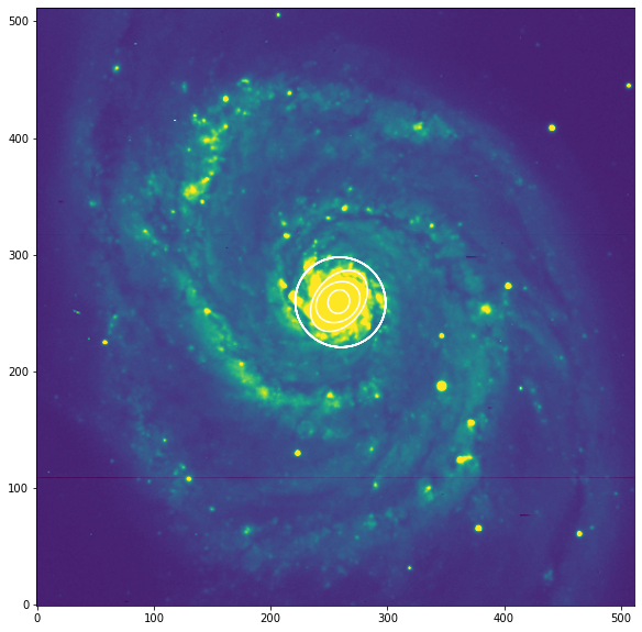
Mostramos los resultados:
[20]:
plt.figure("Galaxia M51", figsize=[10, 10])
plt.imshow(data,vmin=np.nanmin(data), vmax=np.median(data)*5, origin='lower')
smas = np.linspace(10, 100, 10)
for sma in smas:
    iso = isolist.get_closest(sma)
    x, y, = iso.sampled_coordinates()
    plt.plot(x, y, color='white')
plt.show()

Ejecutando Ellipse de una manera más detallada:
Podemos ajustar elipses individuales, simplemente llamando al método fit_isophote en la misma instancia de Ellipse (pasando la longitud del semieje mayor al método):
[21]:
isophote = ellipse.fit_isophote(sma=20.)

isophote.to_table()
[21]:
| sma | intens | intens_err | ellipticity | ellipticity_err | pa | pa_err | grad | grad_error | grad_rerror | x0 | x0_err | y0 | y0_err | ndata | nflag | niter | stop_code |
|---|---|---|---|---|---|---|---|---|---|---|---|---|---|---|---|---|---|
| deg | deg | ||||||||||||||||
| float64 | float64 | float64 | float64 | float64 | float64 | float64 | float64 | float64 | float64 | float64 | float64 | float64 | float64 | int64 | int64 | int64 | int64 |
| 20.0 | 734.422133462885 | 7.140777819896603 | 0.18589782590134635 | 0.017731572121543502 | 34.04174658618836 | 3.037588928039621 | -47.23914015131998 | 5.440605013393248 | 0.11517155045509912 | 257.6759331951344 | 0.2035554607358991 | 259.40038230192096 | 0.19275772890075374 | 114 | 0 | 13 | 0 |
Tenemos que tener en cuenta que en este caso obtenemos una instancia de la clase Isophote, no IsophoteList como antes:
[22]:
type(isophote)
[22]:
photutils.isophote.isophote.Isophote
El algoritmo de ajuste es bastante sensible a las condiciones iniciales de la posición x e y del centro de la galaxia en la imagen. Cuando se usan valores predeterminados como en los ejemplos anteriores, los métodos asumen que la galaxia está exactamente centrada en la imagen, pero esto puede no ser así.
El algoritmo de ajuste también puede fallar en la convergencia si la elipticidad o el ángulo de posición (PA) del semieje mayor están demasiado alejados de los valores reales. Para anular los valores predeterminados, podemos inicializar Ellipse con una instancia de EllipeGeometry.
[23]:
# el usuario define aquí los parámetros de geometría que se utilizarán como primera suposición.
x0 = 256.    # posicion central
y0 = 256.    # posicion central
sma = 20.    # longitud del semieje mayor en pixeles
eps = 0.2    # elipticidad

#el ángulo de posición se define en radianes,
#en sentido antihorario desde el eje +X (girando hacia el eje +Y)
#aquí usamos 35 grados como una primera suposición.

pa = 35. / 180. * np.pi

# tenga en cuenta que EllipseGeometry tiene parámetros adicionales
#con valores predeterminados. Consulte la documentación para obtener más información.
g = EllipseGeometry(x0, y0, sma, eps, pa)

# la geometría personalizada se pasa al constructor Ellipse.
ellipse = Ellipse(data, geometry=g)

# el ajuste procede como de costumbre.
isophote_list = ellipse.fit_image()

isophote_list.to_table()
[23]:
| sma | intens | intens_err | ellipticity | ellipticity_err | pa | pa_err | grad | grad_error | grad_rerror | x0 | x0_err | y0 | y0_err | ndata | nflag | niter | stop_code |
|---|---|---|---|---|---|---|---|---|---|---|---|---|---|---|---|---|---|
| deg | deg | ||||||||||||||||
| float64 | float64 | float64 | float64 | float64 | float64 | float64 | float64 | object | object | float64 | float64 | float64 | float64 | int64 | int64 | int64 | int64 |
| 0.0 | 7596.479535075031 | 0.0 | 0.0 | 0.0 | 0.0 | 0.0 | 0.0 | None | None | 256.8775421921039 | 0.0 | 257.99293482077127 | 0.0 | 1 | 0 | 0 | 0 |
| 0.5346972612827552 | 6849.000160534691 | 23.86989404326559 | 0.03466989553232871 | 0.09256580703288413 | 144.94890713335604 | 80.43485553460222 | -1654.0356760084585 | 649.4095660978811 | 0.3926212569157185 | 256.8775421921039 | 0.025620961180617796 | 257.99293482077127 | 0.025581734732417157 | 13 | 0 | 10 | 0 |
| 0.5881669874110307 | 6772.551100106997 | 27.175831281560043 | 0.04561669085172741 | 0.09642353430251077 | 146.872985239784 | 64.03784333221734 | -1624.8414287781466 | 673.2077602234197 | 0.4143221291013367 | 256.86480233791065 | 0.029607840762342977 | 257.99358486076227 | 0.02941432525172341 | 13 | 0 | 11 | 0 |
| 0.6469836861521338 | 6677.100064615137 | 25.114092353991897 | 0.05274804969197659 | 0.08286778614747728 | 134.5092723447782 | 47.766746521594335 | -1576.7214078942113 | 579.5792847995145 | 0.36758509264713485 | 256.8622624513328 | 0.02799450020404713 | 257.9785445298125 | 0.028005768478022972 | 13 | 0 | 10 | 0 |
| 0.7116820547673471 | 6581.746214780735 | 27.122645979892372 | 0.05999860825128903 | 0.08177539003771511 | 135.06875214861728 | 41.59641637749309 | -1555.1107124551086 | 566.157914653366 | 0.36406277065608555 | 256.8456690013686 | 0.03051449084987157 | 257.9759321630534 | 0.030512216222008767 | 13 | 0 | 10 | 0 |
| 0.7828502602440819 | 6461.437332669412 | 27.45500160009008 | 0.03813043168920357 | 0.07291748421344356 | 160.30302924920312 | 57.71201577377653 | -1587.2995831879064 | 515.6632595797024 | 0.32486826371115957 | 256.8179047348224 | 0.029672434534054 | 257.980613804252 | 0.029487497252663603 | 13 | 0 | 50 | 2 |
| 0.8611352862684901 | 6336.5582156642795 | 30.46710661357744 | 0.03813043168920357 | 0.06797559285889807 | 128.30410789339282 | 53.80070051682559 | -1737.1931043108448 | 490.5059771949739 | 0.28235547100537256 | 256.8179047348224 | 0.030304553830329123 | 257.980613804252 | 0.030361391106634775 | 13 | 0 | 50 | 2 |
| 0.9472488148953392 | 6226.47595235802 | 28.93204171254085 | 0.0814477599712011 | 0.05770037560686564 | 128.30410789339282 | 21.8629125755565 | -1727.0648138775175 | 427.3207736558937 | 0.24742602027569247 | 256.8179047348224 | 0.028821908155805126 | 257.980613804252 | 0.029185350912232906 | 13 | 0 | 10 | 0 |
| 1.0419736963848731 | 6077.486048054 | 27.846385420567998 | 0.09215981065590978 | 0.04293735594344223 | 118.13132060214897 | 14.464965569465349 | -2008.1908960889973 | 351.656406336911 | 0.175111044981715 | 256.80556147520076 | 0.02345005741824789 | 257.98837729637467 | 0.024323933649597226 | 13 | 0 | 10 | 0 |
| ... | ... | ... | ... | ... | ... | ... | ... | ... | ... | ... | ... | ... | ... | ... | ... | ... | ... |
| 16.52892561983471 | 903.9936004928442 | 8.204800823801062 | 0.3225039240020763 | 0.02801100665604879 | 49.899883148431506 | 2.9898235744414987 | -35.029068543638374 | 7.187249093582541 | 0.2051795663544076 | 258.7324943036067 | 0.2805393954406921 | 259.5451981925187 | 0.29431473144322967 | 85 | 0 | 10 | 0 |
| 18.18181818181818 | 815.0024222916826 | 9.294165720968845 | 0.18559930755829573 | 0.02368552913658422 | 39.2366822408665 | 4.041456710808486 | -50.81055123269196 | 6.883415235147378 | 0.13547216214254587 | 258.6455645149596 | 0.24376550195329003 | 259.7756290052206 | 0.23650316303386393 | 103 | 0 | 10 | 0 |
| 20.0 | 734.8346125341519 | 7.188060790473552 | 0.18616832014714121 | 0.0179475315551449 | 35.027618596512454 | 3.07020165552574 | -47.04174983357989 | 5.443273544588005 | 0.11571154482655796 | 257.67559213697655 | 0.20557935370742536 | 259.35862654987864 | 0.19558140941606694 | 114 | 0 | 20 | 0 |
| 22.0 | 671.4751472538611 | 8.009096180360883 | 0.22823881209348726 | 0.025074956383398298 | 36.637710765256266 | 3.5621204078837554 | -32.366025962849 | 5.437001106337736 | 0.16798482188015731 | 257.1638921170691 | 0.3256187708559168 | 258.8748275240517 | 0.3081391866781498 | 121 | 0 | 10 | 0 |
| 24.200000000000003 | 656.4254786803965 | 9.188646212028601 | 0.29437310612156253 | 0.015279790429643843 | 40.092733440480266 | 1.7529550214694376 | -50.65360142752443 | 4.943325838887158 | 0.09759080696285943 | 256.45325154895875 | 0.22877550689765366 | 258.139752899959 | 0.21905809491665024 | 127 | 0 | 10 | 0 |
| 26.620000000000005 | 470.6411159435701 | 6.300172384963755 | 0.18365530946759712 | 0.02489052075207591 | 35.19763723121675 | 4.287437316885469 | -22.279435263560185 | 3.4188204524740886 | 0.15345184525686095 | 256.9491684341771 | 0.3781636080845221 | 257.5506810512856 | 0.35964932181735776 | 151 | 0 | 10 | 0 |
| 29.282000000000007 | 513.0132274268149 | 7.126751425724801 | 0.3032105722257286 | 0.014328501055925346 | 50.86371283785065 | 1.6078132886700334 | -33.94065571069158 | 3.326903735611407 | 0.09802119805727282 | 258.5768125612312 | 0.24930555337303292 | 260.3329111292059 | 0.2629141304399094 | 153 | 0 | 17 | 0 |
| 32.21020000000001 | 335.1372695983853 | 5.500207429045783 | 0.01846737039281754 | 0.03404910325758143 | 140.86371283785067 | 53.44106317495372 | -13.596010529993583 | 2.5081832026010886 | 0.18447935128234064 | 259.75594669916933 | 0.5548318227838185 | 259.37341418002023 | 0.5535325557811654 | 201 | 0 | 50 | 2 |
| 35.43122000000001 | 291.34424776106533 | 5.91747217135161 | 0.01846737039281754 | 0.06423218869894584 | 140.86371283785067 | 100.7708265706513 | -6.940407851315642 | 2.4454690150336176 | 0.35235234980751856 | 259.75594669916933 | 1.1511406450664645 | 259.37341418002023 | 1.148342182466996 | 221 | 0 | 3 | 5 |
| 38.974342000000014 | 266.75353601409614 | 6.329196693479066 | 0.01846737039281754 | 0.1885115482314048 | 140.86371283785067 | 296.7824343641862 | -2.054837020912551 | 2.645863647595697 | 1.2876270091827875 | 259.75594669916933 | 3.7213184713692375 | 259.37341418002023 | 3.714961780205796 | 244 | 0 | 8 | 5 |
Graficando
[24]:
import matplotlib.pyplot as plt
plt.rcParams['image.origin'] = 'lower'
Los atributos de una instancia de Isophote también son atributos de una instancia de IsophoteList. La diferencia es que, mientras que las isófotas individuales tienen atributos escalares, los mismos atributos en una IsophoteList son matrices numpy que almacenan el atributo dado en todas las isófotas de la lista. Por lo tanto, los atributos en una IsophoteList se pueden usar directamente como parámetros para matplotlib.
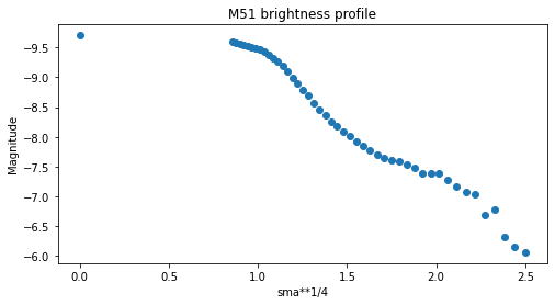
Como ejemplo, un gráfico básico de magnitud en función de la longitud del semieje mayor se puede hacer simplemente como:
[25]:
plt.figure(figsize=(8, 4))

plt.scatter(isophote_list.sma**0.25, -2.5*np.log10(isophote_list.intens))
plt.title("M51 brightness profile")
plt.xlabel('sma**1/4')
plt.ylabel('Magnitude')
plt.gca().invert_yaxis()
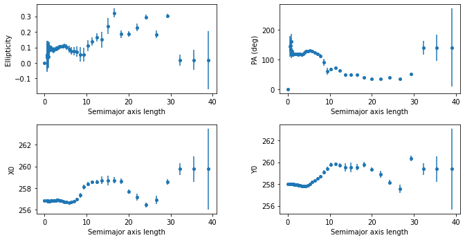
A continuación podemos ver un gráfico que representa la geometría de la elipse en función de la longitud del semieje mayor:
[26]:
plt.figure(figsize=(10, 5))
plt.figure(1)

plt.subplot(221)
plt.errorbar(isophote_list.sma, isophote_list.eps, yerr=isophote_list.ellip_err, fmt='o', markersize=4)
plt.xlabel('Semimajor axis length')
plt.ylabel('Ellipticity')

plt.subplot(222)
plt.errorbar(isophote_list.sma, isophote_list.pa/np.pi*180., yerr=isophote_list.pa_err/np.pi* 80., fmt='o', markersize=4)
plt.xlabel('Semimajor axis length')
plt.ylabel('PA (deg)')

plt.subplot(223)
plt.errorbar(isophote_list.sma, isophote_list.x0, yerr=isophote_list.x0_err, fmt='o', markersize=4)
plt.xlabel('Semimajor axis length')
plt.ylabel('X0')

plt.subplot(224)
plt.errorbar(isophote_list.sma, isophote_list.y0, yerr=isophote_list.y0_err, fmt='o', markersize=4)
plt.xlabel('Semimajor axis length')
plt.ylabel('Y0')

plt.subplots_adjust(top=0.92, bottom=0.08, left=0.10, right=0.95, hspace=0.35, wspace=0.35)
[27]:
plt.figure("Galaxia M51", figsize=[10, 10])
plt.imshow(data,vmin=np.nanmin(data), vmax=np.median(data)*5, origin='lower')
smas = np.linspace(10, 100, 10)
for sma in smas:
    iso = isophote_list.get_closest(sma)
    x, y, = iso.sampled_coordinates()
    plt.plot(x, y, color='white')
plt.show()
El algoritmo de ajuste asume que una distribución uniforme del brillo superficial dominará la imagen y este no es el mejor caso ya que M51 tiene muchas regiones de formación de estrellas.
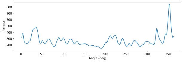
Podemos examinar la muestra de brillo elíptica asociada con la elipse que se muestra arriba para tener una idea de lo que está pasando. El siguiente gráfico muestra una gran contaminación de esas regiones HII brillantes.
[28]:
plt.figure(figsize=(10, 3))
plt.plot(iso.sample.values[0] / np.pi*180., iso.sample.values[2])
plt.ylabel("Intensity")
plt.xlabel("Angle (deg)")
[28]:
Text(0.5, 0, 'Angle (deg)')
Podemos usar sigma-clipping para tratar de mitigarlos.
Ejecutando Ellipse con sigma-clipping
[29]:
from photutils.isophote import Ellipse
ellipse = Ellipse(data, geometry=g)
El recorte de Sigma se implementa a través de parámetros en el método fit_image. En este ejemplo, debido a la importante contaminación de la imagen por elementos no elípticos, aplicamos un recorte bastante agresivo.
[30]:
isophote_list = ellipse.fit_image(sclip=2., nclip=3)
isophote_list.to_table()
[30]:
| sma | intens | intens_err | ellipticity | ellipticity_err | pa | pa_err | grad | grad_error | grad_rerror | x0 | x0_err | y0 | y0_err | ndata | nflag | niter | stop_code |
|---|---|---|---|---|---|---|---|---|---|---|---|---|---|---|---|---|---|
| deg | deg | ||||||||||||||||
| float64 | float64 | float64 | float64 | float64 | float64 | float64 | float64 | object | object | float64 | float64 | float64 | float64 | int64 | int64 | int64 | int64 |
| 0.0 | 7600.780179543361 | 0.0 | 0.0 | 0.0 | 0.0 | 0.0 | 0.0 | None | None | 256.8859385456823 | 0.0 | 257.98953468113984 | 0.0 | 1 | 0 | 0 | 0 |
| 0.5346972612827552 | 6852.6807100935885 | 20.692033269302982 | 0.04799573249878426 | 0.08168375281229916 | 155.67248001538843 | 51.622419201190525 | -1600.1956911555108 | 584.7874621128432 | 0.3654474670473364 | 256.8859385456823 | 0.022889268334231924 | 257.98953468113984 | 0.022612742986566056 | 13 | 0 | 50 | 0 |
| 0.5881669874110307 | 6765.202337922748 | 23.86340150284385 | 0.04414254671731125 | 0.05789510926236029 | 139.9160055076753 | 39.70389279859427 | -2378.228949657796 | 474.949982369577 | 0.19970742616597856 | 256.8716368552103 | 0.017723390884621163 | 257.98117950905566 | 0.01767999134520011 | 13 | 0 | 10 | 0 |
| 0.6469836861521338 | 6630.765030253545 | 12.320765527433458 | 0.0544804439186206 | 0.0427309982116427 | 146.20262255962308 | 27.54679980163171 | -1641.4437959635475 | 299.57813300121654 | 0.18250891912224174 | 256.8660598692693 | 0.015363370740489312 | 257.98158842819157 | 0.015202707576202429 | 10 | 3 | 10 | 0 |
| 0.7116820547673471 | 6575.021821215169 | 21.220174559525383 | 0.08185784694155247 | 0.06342699384849047 | 167.7621282353217 | 24.940881547754714 | -1575.9650693889798 | 439.5866975659199 | 0.27893175179089014 | 256.83084532234335 | 0.024426165057937023 | 258.01400293328055 | 0.024566435770082867 | 12 | 1 | 10 | 0 |
| 0.7828502602440819 | 6467.577748797088 | 21.124397771814653 | 0.08757556356135573 | 0.056274193112099795 | 165.046171505206 | 20.714748397118147 | -1597.7398682084472 | 387.8245303308215 | 0.24273321211273952 | 256.81703622821766 | 0.023829316360574854 | 258.0142048559859 | 0.023965163985755652 | 12 | 1 | 10 | 0 |
| 0.8611352862684901 | 6349.139670056983 | 23.22393813214937 | 0.08813547501834287 | 0.050389929304796126 | 160.0144792321436 | 18.469394837894527 | -1781.3091980813267 | 370.31063908871386 | 0.20788678320842932 | 256.80848215840496 | 0.02348578883047456 | 258.0112620534792 | 0.023600963982566447 | 12 | 1 | 10 | 0 |
| 0.9472488148953392 | 6221.610370912634 | 28.830935033856743 | 0.07617565911498689 | 0.057641846554700164 | 128.34649223232708 | 23.28619267887906 | -1733.7445527313566 | 426.767597920302 | 0.2461536777421844 | 256.81808841198216 | 0.028724188114443775 | 257.98001644561504 | 0.029043039496036017 | 13 | 0 | 10 | 0 |
| 1.0419736963848731 | 6057.037687525787 | 17.797972461776382 | 0.10665157437084688 | 0.026132750559961764 | 118.74500572076485 | 9.147872590373101 | -2016.0041959581501 | 199.12943372591985 | 0.09877431511558894 | 256.81516146263283 | 0.015848918173123772 | 257.97259034682435 | 0.015804893557838644 | 11 | 2 | 50 | 2 |
| ... | ... | ... | ... | ... | ... | ... | ... | ... | ... | ... | ... | ... | ... | ... | ... | ... | ... |
| 57.06233412220004 | 183.93894607873287 | 0.8911314521483652 | 0.21959824295943495 | 0.00720694688376061 | 162.58452846813097 | 1.1066090541867246 | -4.753332443595598 | 0.23508741794536095 | 0.049457390311949664 | 253.02745580897522 | 0.2546832745527912 | 261.1373134474524 | 0.22250209999595955 | 279 | 38 | 10 | 0 |
| 62.76856753442005 | 157.0244941004311 | 1.0149208687004487 | 0.21959824295943495 | 0.004167881105068473 | 162.58452846813097 | 0.6238923500962802 | -7.207668365191359 | None | None | 253.02745580897522 | 0.15856412386415936 | 261.1373134474524 | 0.14096889845071753 | 318 | 31 | 3 | 5 |
| 69.04542428786206 | 165.79368789450075 | 0.7264367433184951 | 0.15447073859174187 | 0.008926197652032388 | 81.05608919547127 | 1.8575074622314105 | -2.8093063908585347 | 0.15752904435623916 | 0.056073999215193356 | 254.6965510636437 | 0.3164628867224775 | 277.08923038378214 | 0.3659384628038651 | 334 | 66 | 28 | 0 |
| 75.94996671664828 | 144.71859938538273 | 0.7608276924745618 | 0.15447073859174187 | 0.03714030846120695 | 81.05608919547127 | 7.767147404457842 | -0.5666023941836529 | 0.14697065573281967 | 0.259389401177119 | 256.44800470812476 | 1.4644037716356266 | 276.67032190538566 | 1.6707852839520463 | 406 | 34 | 50 | 2 |
| 83.5449633883131 | 140.4171097907267 | 0.8168243384497106 | 0.15447073859174187 | 0.02263071032627645 | 81.05608919547127 | 4.646490356310346 | -0.869065391729032 | 0.1518228138087035 | 0.1746966514299314 | 256.44800470812476 | 0.9764090336713479 | 276.67032190538566 | 1.1059134518090457 | 451 | 33 | 12 | 5 |
| 91.89945972714443 | 163.24876033978921 | 0.8375614566366035 | 0.42106144265922074 | 0.009096907633427893 | 67.53639446553697 | 0.7781879295380345 | -1.6924032692542894 | 0.15111164232613994 | 0.08928820043743067 | 253.05232962002236 | 0.4856739336157087 | 241.6656158497913 | 0.6252457771719298 | 369 | 65 | 19 | 0 |
| 101.08940569985889 | 159.363569930879 | 0.8647118417724167 | 0.4533274239046324 | 0.008613639616144995 | 75.96416641159895 | 0.6727079741554495 | -1.6247192810526305 | 0.13020344623860522 | 0.08013904171448523 | 254.69158827308448 | 0.48350220190127097 | 249.95153241956768 | 0.6868838368430331 | 373 | 89 | 50 | 2 |
| 111.19834626984479 | 137.33399834679125 | 0.814892568064858 | 0.28425475070329853 | 0.010715070024485733 | 56.162753417478285 | 1.3876873632722189 | -1.342605543510599 | 0.0941734402617292 | 0.07014229958822285 | 252.77804186925772 | 0.71215605777498 | 252.81666870500646 | 0.7929524175114182 | 504 | 86 | 10 | 0 |
| 122.31818089682928 | 122.40423192438517 | 0.6577024332392916 | 0.28425475070329853 | 0.01443552988012702 | 56.162753417478285 | 1.9585886075503005 | -0.6492589235395249 | 0.07856938490424463 | 0.12101394691029083 | 252.77804186925772 | 1.078722335283315 | 252.81666870500646 | 1.187545113201799 | 551 | 98 | 1 | 5 |
| 134.5499989865122 | 114.46261257104743 | 0.7007407741077802 | 0.28425475070329853 | 0.03930694485169253 | 56.162753417478285 | 5.195611772322989 | 0.20833943901232954 | None | None | 252.77804186925772 | 3.1929865229597567 | 252.81666870500646 | 3.4785300715225027 | 622 | 92 | 4 | 5 |
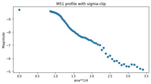
Observamos cómo la estabilidad añadida proporcionada por el sigma-clipping permite que el ajuste se haga mayor antes de detectar una condición de señal/ruido demasiado baja.
[31]:
plt.figure(figsize=(8, 4))

plt.scatter(isophote_list.sma**0.25, -2.5*np.log10(isophote_list.intens))
plt.title("M51 profile with sigma-clip")
plt.xlabel('sma**1/4')
plt.ylabel('Magnitude')
plt.gca().invert_yaxis()
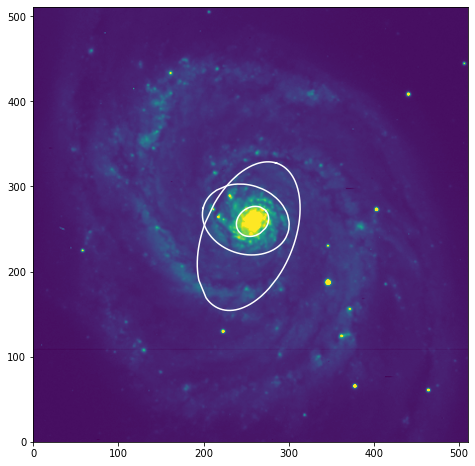
Algunas de las isófotas en la imagen:
[32]:
fig, ax = plt.subplots(figsize=(8, 8))
ax.imshow(data, vmin=0, vmax=1000)
plt.axis([0, 511, 0, 511])

isos = []
smas = [20., 50., 90.]
for sma in smas:
    iso = isophote_list.get_closest(sma)
    isos.append(iso)
    x, y, = iso.sampled_coordinates()
    plt.plot(x, y, color='white')
[33]:
plt.figure(figsize=(10, 3))

for iso in isos:
    angles = ((iso.sample.values[0] + iso.sample.geometry.pa) / np.pi*180.) % 360.
    plt.scatter(angles, iso.sample.values[2], label=f"isofota {np.round(iso.sma, 2)}")

plt.xlabel("Angle (deg)")
plt.ylabel("Intensity")
plt.legend(loc='upper right')
[33]:
<matplotlib.legend.Legend at 0x7f669a5d6550>

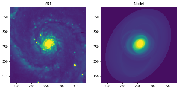
Construcción de un modelo de imagen a partir de los resultados obtenidos por el ajuste Ellipse
Inicialmente ajustamos la imagen de prueba M51. Luego, a partir de los resultados de ajuste construimos una imagen modelo. Finalmente, restamos la imagen del modelo de la imagen original.
[34]:
from photutils.isophote import Ellipse
ellipse = Ellipse(data, geometry=g)
isophote_list = ellipse.fit_image(sclip=2., nclip=3)
Ahora construimos una imagen modelo.
[35]:
import numpy as np
from photutils.isophote import build_ellipse_model

model_image = build_ellipse_model(data.shape, isophote_list, fill=np.mean(data[0:10, 0:10]))
Gráfico de la región modelada:
[36]:
import matplotlib
import matplotlib.pyplot as plt

fig, (ax1, ax2) = plt.subplots(1, 2, figsize=(10, 10))
limits = [128, 384]

ax1.imshow(data, vmin=0, vmax=1000)
ax1.set_title("M51")
ax1.set_xlim(limits)
ax1.set_ylim(limits)

ax2.imshow(model_image, vmin=0, vmax=1000)
ax2.set_title("Model")
ax2.set_xlim(limits)
ax2.set_ylim(limits)
plt.show()
Test de galaxia elíptica M105
Elegimos una imagen de dominio público de M105 tal como se publicó en asd.gsfc.nasa.gov.
[37]:
url = 'https://github.com/astropy/photutils-datasets/raw/main/data/isophote/M105-S001-RGB.fits'
path = download_file(url)
hdu = fits.open(path)
data = hdu[0].data[0]
hdu.close()
Repetimos el procedimiento anterior pero esta vez pasando una instancia de EllipseGeometry al constructor Ellipse, ya que el centro de la galaxia no coincide con el centro de la imagen. También pasamos valores de primera estimación para los parámetros de ángulo de posición y elipticidad, obtenidos de la inspección visual de la imagen.
[38]:
from photutils.isophote import Ellipse, EllipseGeometry, build_ellipse_model
g = EllipseGeometry(530., 511, 10., 0.1, 10./180.*np.pi)
g.find_center(data)

ellipse = Ellipse(data, geometry=g)
isolist = ellipse.fit_image()
isophote_list.to_table()
INFO: Found center at x0 = 530.0, y0 = 512.0 [photutils.isophote.geometry]
[38]:
| sma | intens | intens_err | ellipticity | ellipticity_err | pa | pa_err | grad | grad_error | grad_rerror | x0 | x0_err | y0 | y0_err | ndata | nflag | niter | stop_code |
|---|---|---|---|---|---|---|---|---|---|---|---|---|---|---|---|---|---|
| deg | deg | ||||||||||||||||
| float64 | float64 | float64 | float64 | float64 | float64 | float64 | float64 | object | object | float64 | float64 | float64 | float64 | int64 | int64 | int64 | int64 |
| 0.0 | 7600.780179543361 | 0.0 | 0.0 | 0.0 | 0.0 | 0.0 | 0.0 | None | None | 256.8859385456823 | 0.0 | 257.98953468113984 | 0.0 | 1 | 0 | 0 | 0 |
| 0.5346972612827552 | 6852.6807100935885 | 20.692033269302982 | 0.04799573249878426 | 0.08168375281229916 | 155.67248001538843 | 51.622419201190525 | -1600.1956911555108 | 584.7874621128432 | 0.3654474670473364 | 256.8859385456823 | 0.022889268334231924 | 257.98953468113984 | 0.022612742986566056 | 13 | 0 | 50 | 0 |
| 0.5881669874110307 | 6765.202337922748 | 23.86340150284385 | 0.04414254671731125 | 0.05789510926236029 | 139.9160055076753 | 39.70389279859427 | -2378.228949657796 | 474.949982369577 | 0.19970742616597856 | 256.8716368552103 | 0.017723390884621163 | 257.98117950905566 | 0.01767999134520011 | 13 | 0 | 10 | 0 |
| 0.6469836861521338 | 6630.765030253545 | 12.320765527433458 | 0.0544804439186206 | 0.0427309982116427 | 146.20262255962308 | 27.54679980163171 | -1641.4437959635475 | 299.57813300121654 | 0.18250891912224174 | 256.8660598692693 | 0.015363370740489312 | 257.98158842819157 | 0.015202707576202429 | 10 | 3 | 10 | 0 |
| 0.7116820547673471 | 6575.021821215169 | 21.220174559525383 | 0.08185784694155247 | 0.06342699384849047 | 167.7621282353217 | 24.940881547754714 | -1575.9650693889798 | 439.5866975659199 | 0.27893175179089014 | 256.83084532234335 | 0.024426165057937023 | 258.01400293328055 | 0.024566435770082867 | 12 | 1 | 10 | 0 |
| 0.7828502602440819 | 6467.577748797088 | 21.124397771814653 | 0.08757556356135573 | 0.056274193112099795 | 165.046171505206 | 20.714748397118147 | -1597.7398682084472 | 387.8245303308215 | 0.24273321211273952 | 256.81703622821766 | 0.023829316360574854 | 258.0142048559859 | 0.023965163985755652 | 12 | 1 | 10 | 0 |
| 0.8611352862684901 | 6349.139670056983 | 23.22393813214937 | 0.08813547501834287 | 0.050389929304796126 | 160.0144792321436 | 18.469394837894527 | -1781.3091980813267 | 370.31063908871386 | 0.20788678320842932 | 256.80848215840496 | 0.02348578883047456 | 258.0112620534792 | 0.023600963982566447 | 12 | 1 | 10 | 0 |
| 0.9472488148953392 | 6221.610370912634 | 28.830935033856743 | 0.07617565911498689 | 0.057641846554700164 | 128.34649223232708 | 23.28619267887906 | -1733.7445527313566 | 426.767597920302 | 0.2461536777421844 | 256.81808841198216 | 0.028724188114443775 | 257.98001644561504 | 0.029043039496036017 | 13 | 0 | 10 | 0 |
| 1.0419736963848731 | 6057.037687525787 | 17.797972461776382 | 0.10665157437084688 | 0.026132750559961764 | 118.74500572076485 | 9.147872590373101 | -2016.0041959581501 | 199.12943372591985 | 0.09877431511558894 | 256.81516146263283 | 0.015848918173123772 | 257.97259034682435 | 0.015804893557838644 | 11 | 2 | 50 | 2 |
| ... | ... | ... | ... | ... | ... | ... | ... | ... | ... | ... | ... | ... | ... | ... | ... | ... | ... |
| 57.06233412220004 | 183.93894607873287 | 0.8911314521483652 | 0.21959824295943495 | 0.00720694688376061 | 162.58452846813097 | 1.1066090541867246 | -4.753332443595598 | 0.23508741794536095 | 0.049457390311949664 | 253.02745580897522 | 0.2546832745527912 | 261.1373134474524 | 0.22250209999595955 | 279 | 38 | 10 | 0 |
| 62.76856753442005 | 157.0244941004311 | 1.0149208687004487 | 0.21959824295943495 | 0.004167881105068473 | 162.58452846813097 | 0.6238923500962802 | -7.207668365191359 | None | None | 253.02745580897522 | 0.15856412386415936 | 261.1373134474524 | 0.14096889845071753 | 318 | 31 | 3 | 5 |
| 69.04542428786206 | 165.79368789450075 | 0.7264367433184951 | 0.15447073859174187 | 0.008926197652032388 | 81.05608919547127 | 1.8575074622314105 | -2.8093063908585347 | 0.15752904435623916 | 0.056073999215193356 | 254.6965510636437 | 0.3164628867224775 | 277.08923038378214 | 0.3659384628038651 | 334 | 66 | 28 | 0 |
| 75.94996671664828 | 144.71859938538273 | 0.7608276924745618 | 0.15447073859174187 | 0.03714030846120695 | 81.05608919547127 | 7.767147404457842 | -0.5666023941836529 | 0.14697065573281967 | 0.259389401177119 | 256.44800470812476 | 1.4644037716356266 | 276.67032190538566 | 1.6707852839520463 | 406 | 34 | 50 | 2 |
| 83.5449633883131 | 140.4171097907267 | 0.8168243384497106 | 0.15447073859174187 | 0.02263071032627645 | 81.05608919547127 | 4.646490356310346 | -0.869065391729032 | 0.1518228138087035 | 0.1746966514299314 | 256.44800470812476 | 0.9764090336713479 | 276.67032190538566 | 1.1059134518090457 | 451 | 33 | 12 | 5 |
| 91.89945972714443 | 163.24876033978921 | 0.8375614566366035 | 0.42106144265922074 | 0.009096907633427893 | 67.53639446553697 | 0.7781879295380345 | -1.6924032692542894 | 0.15111164232613994 | 0.08928820043743067 | 253.05232962002236 | 0.4856739336157087 | 241.6656158497913 | 0.6252457771719298 | 369 | 65 | 19 | 0 |
| 101.08940569985889 | 159.363569930879 | 0.8647118417724167 | 0.4533274239046324 | 0.008613639616144995 | 75.96416641159895 | 0.6727079741554495 | -1.6247192810526305 | 0.13020344623860522 | 0.08013904171448523 | 254.69158827308448 | 0.48350220190127097 | 249.95153241956768 | 0.6868838368430331 | 373 | 89 | 50 | 2 |
| 111.19834626984479 | 137.33399834679125 | 0.814892568064858 | 0.28425475070329853 | 0.010715070024485733 | 56.162753417478285 | 1.3876873632722189 | -1.342605543510599 | 0.0941734402617292 | 0.07014229958822285 | 252.77804186925772 | 0.71215605777498 | 252.81666870500646 | 0.7929524175114182 | 504 | 86 | 10 | 0 |
| 122.31818089682928 | 122.40423192438517 | 0.6577024332392916 | 0.28425475070329853 | 0.01443552988012702 | 56.162753417478285 | 1.9585886075503005 | -0.6492589235395249 | 0.07856938490424463 | 0.12101394691029083 | 252.77804186925772 | 1.078722335283315 | 252.81666870500646 | 1.187545113201799 | 551 | 98 | 1 | 5 |
| 134.5499989865122 | 114.46261257104743 | 0.7007407741077802 | 0.28425475070329853 | 0.03930694485169253 | 56.162753417478285 | 5.195611772322989 | 0.20833943901232954 | None | None | 252.77804186925772 | 3.1929865229597567 | 252.81666870500646 | 3.4785300715225027 | 622 | 92 | 4 | 5 |
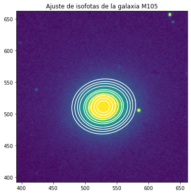
[39]:
fig, (ax1) = plt.subplots(figsize=(14, 5), nrows=1, ncols=1)
fig.subplots_adjust(left=0.04, right=0.98, bottom=0.02, top=0.98)
ax1.imshow(data, vmin=1464., vmax=1480.)
ax1.set_title('Ajuste de isofotas de la galaxia M105')
limits = [512-120, 512+150]
ax1.set_xlim(limits)
ax1.set_ylim(limits)

smas = np.linspace(10, 50, 10)
for sma in smas:
    iso = isolist.get_closest(sma)
    x, y, = iso.sampled_coordinates()
    ax1.plot(x, y, color='white')
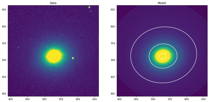
Construimos una imagen modelo
[40]:
fill = np.mean(data[20:120, 20:120])
model_image = build_ellipse_model(data.shape, isolist, fill=fill)
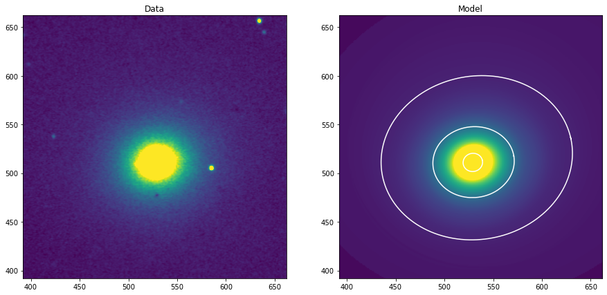
[41]:
fig, (ax1, ax2) = plt.subplots(1, 2, figsize=(15, 10))
limits = [512-120, 512+150]
ax1.imshow(data, vmin=1464., vmax=1480.)
ax1.set_xlim(limits)
ax1.set_ylim(limits)
ax1.set_title("Data")

ax2.imshow(model_image, vmin=1464., vmax=1480.)
ax2.set_xlim(limits)
ax2.set_ylim(limits)
ax2.set_title("Model")


# overplot a few isophotes on the residual map
iso1 = isolist.get_closest(10.)
iso2 = isolist.get_closest(40.)
iso3 = isolist.get_closest(100.)

plt.axis([512-120, 512+150, 512-120, 512+150])
x, y, = iso1.sampled_coordinates()
plt.plot(x, y, color='white')
x, y, = iso2.sampled_coordinates()
plt.plot(x, y, color='white')
x, y, = iso3.sampled_coordinates()
plt.plot(x, y, color='white')
[41]:
[<matplotlib.lines.Line2D at 0x7f6698eb73a0>]
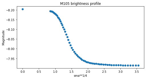
Comprobamos cómo quedan los perfiles radiales.
[42]:
plt.figure(figsize=(8, 4))

plt.scatter(isolist.sma**0.25, -2.5*np.log10(isolist.intens))
plt.title("M105 brightness profile")
plt.xlabel('sma**1/4')
plt.ylabel('Magnitude')
plt.gca().invert_yaxis()
[43]:
plt.figure(figsize=(10, 5))
plt.figure(1)

plt.subplot(221)
plt.errorbar(isolist.sma, isolist.eps, yerr=isolist.ellip_err, fmt='o', markersize=4)
plt.xlabel('Semimajor axis length')
plt.ylabel('Ellipticity')

plt.subplot(222)
plt.errorbar(isolist.sma, isolist.pa/np.pi*180., yerr=isolist.pa_err/np.pi* 80., fmt='o', markersize=4)
plt.xlabel('Semimajor axis length')
plt.ylabel('PA (deg)')

plt.subplot(223)
plt.errorbar(isolist.sma, isolist.x0, yerr=isolist.x0_err, fmt='o', markersize=4)
plt.xlabel('Semimajor axis length')
plt.ylabel('X0')

plt.subplot(224)
plt.errorbar(isolist.sma, isolist.y0, yerr=isolist.y0_err, fmt='o', markersize=4)
plt.xlabel('Semimajor axis length')
plt.ylabel('Y0')

plt.subplots_adjust(top=0.92, bottom=0.08, left=0.10, right=0.95, hspace=0.35, wspace=0.35)
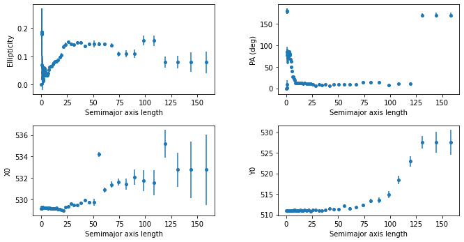
Podemos observar cómo la presencia de la estrella brillante hace que aparezca un componente no elíptica alrededor de una longitud del semieje mayor de \(\sim 50\) píxeles.
Repitamos el procedimiento con el recorte sigma habilitado para eliminar la estrella y ver el efecto en la imagen residual.
Tenga en cuenta que no es necesario crear una nueva instancia de Ellipse, ya que nada cambió ni en el mapa de píxeles de entrada ni en la geometría de la elipse de entrada.
[44]:
isolist2 = ellipse.fit_image(sclip=3., nclip=3)

fill = np.mean(data[20:120, 20:120])
model_image2 = build_ellipse_model(data.shape, isolist2, fill=fill)
[45]:
fig, (ax1, ax2) = plt.subplots(1, 2, figsize=(15, 10))
limits = [512-120, 512+150]
ax1.imshow(data, vmin=1464., vmax=1480.)
ax1.set_xlim(limits)
ax1.set_ylim(limits)
ax1.set_title("Data")

ax2.imshow(model_image2, vmin=1464., vmax=1480.)
ax2.set_xlim(limits)
ax2.set_ylim(limits)
ax2.set_title("Model")


# overplot a few isophotes on the residual map
iso1 = isolist2.get_closest(10.)
iso2 = isolist2.get_closest(40.)
iso3 = isolist2.get_closest(100.)

plt.axis([512-120, 512+150, 512-120, 512+150])
x, y, = iso1.sampled_coordinates()
plt.plot(x, y, color='white')
x, y, = iso2.sampled_coordinates()
plt.plot(x, y, color='white')
x, y, = iso3.sampled_coordinates()
plt.plot(x, y, color='white')
[45]:
[<matplotlib.lines.Line2D at 0x7f669a4863a0>]
[46]:
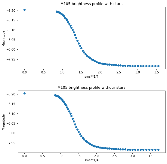
plt.figure(figsize=(8, 8))
plt.figure(1)

plt.subplot(211)
plt.scatter(isolist.sma**0.25, -2.5*np.log10(isolist.intens))
plt.title("M105 brightness profile with stars")
plt.xlabel('sma**1/4')
plt.ylabel('Magnitude')
plt.gca().invert_yaxis()

plt.subplot(212)
plt.scatter(isolist2.sma**0.25, -2.5*np.log10(isolist2.intens))
plt.title("M105 brightness profile withour stars")
plt.xlabel('sma**1/4')
plt.ylabel('Magnitude')
plt.gca().invert_yaxis()

plt.subplots_adjust(top=0.92, bottom=0.08, left=0.10, right=0.95, hspace=0.35, wspace=0.35)
[47]:
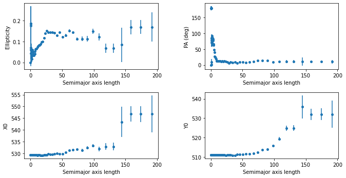
plt.figure(figsize=(10, 5))
plt.figure(1)

plt.subplot(221)
plt.errorbar(isolist2.sma, isolist2.eps, yerr=isolist2.ellip_err, fmt='o', markersize=4)
plt.xlabel('Semimajor axis length')
plt.ylabel('Ellipticity')

plt.subplot(222)
plt.errorbar(isolist2.sma, isolist2.pa/np.pi*180., yerr=isolist2.pa_err/np.pi* 80., fmt='o', markersize=4)
plt.xlabel('Semimajor axis length')
plt.ylabel('PA (deg)')

plt.subplot(223)
plt.errorbar(isolist2.sma, isolist2.x0, yerr=isolist2.x0_err, fmt='o', markersize=4)
plt.xlabel('Semimajor axis length')
plt.ylabel('X0')

plt.subplot(224)
plt.errorbar(isolist2.sma, isolist2.y0, yerr=isolist2.y0_err, fmt='o', markersize=4)
plt.xlabel('Semimajor axis length')
plt.ylabel('Y0')

plt.subplots_adjust(top=0.92, bottom=0.08, left=0.10, right=0.95, hspace=0.35, wspace=0.35)
Análisis del brillo superficial de la galaxia espiral NGC 628
Distribución del brillo superficial: ellipse fitting
[48]:
url_g = 'https://dr9.sdss.org/sas/dr9/boss/photoObj/frames/301/7845/2/frame-g-007845-2-0104.fits.bz2'
url_r = 'https://dr9.sdss.org/sas/dr9/boss/photoObj/frames/301/7845/2/frame-r-007845-2-0104.fits.bz2'
[49]:
from astropy.utils.data import download_file

#path_g = download_file(url_g)
#path_r = download_file(url_r)
Abrimos nuestras imagenes de la galaxias M78 del catalogo SDSS en las bandas G y R.
[50]:
from astropy.io import fits
path_g = 'imagenes/isofotas/g.fit'
path_r = 'imagenes/isofotas/r.fit'

g_hdu = fits.open(path_g)
g_header = g_hdu[0].header
g_data = g_hdu[0].data
g_hdu.close()

r_hdu = fits.open(path_r)
r_header = r_hdu[0].header
r_data = r_hdu[0].data
r_hdu.close()
[51]:
g_header
[51]:
SIMPLE  =                    T /
BITPIX  =                  -32 / 32 bit floating point
NAXIS   =                    2
NAXIS1  =                 2048
NAXIS2  =                 1489
EXTEND  =                    T /Extensions may be present
BZERO   =              0.00000 /Set by MRD_SCALE
BSCALE  =              1.00000 /Set by MRD_SCALE
TAI     =        4735092988.65 / 1st row Number of seconds since Nov 17 1858
RA      =            24.903097 / 1st row RA of telescope boresight (deg)
DEC     =            16.513296 / 1st row Dec of telescope boresight (degrees)
SPA     =              95.876  / 1st row Cam col position angle wrt N (deg)
IPA     =              34.842  / 1st row Inst rotator position angle (deg)
IPARATE =              0.0015  / 1st row Inst rotator anglr velocity (deg/sec)
AZ      =            273.35022 / 1st row Azimuth (encoder) of tele (0=N?) (deg)
ALT     =            36.699549 / 1st row Altitude (encoder) of tele (degrees)
FOCUS   =           -131.50000 / 1st row - Focus piston (microns?)
DATE-OBS= '2008-12-04'         / 1st row - TAI date
TAIHMS  = '07:36:28.64'        / 1st row TAI time HH:MM:SS.SS
COMMENT  TAI,RA,DEC,SPA,IPA,IPARATE,AZ,ALT,FOCUS at reading of col 0, row 0
ORIGIN  = 'SDSS    '
TELESCOP= '2.5m    '
TIMESYS = 'TAI     '
RUN     =                 7845 / Run number
FRAME   =                  112 / Frame sequence number within the run
CCDLOC  =                   52 / Survey location of CCD (e.g., rowCol)
STRIPE  =                   75 / Stripe index number (23 <--> eta=0)
STRIP   = 'S       '           / Strip in the stripe being tracked.
FLAVOR  = 'science '           / Flavor of this run
OBSERVER= 'asimmons'           / Observer
SYS_SCN = 'mean    '           / System of the scan great circle (e.g., mean)
EQNX_SCN=           2000.00    / Equinox of the scan great circle. (years)
NODE    =           95.00000   / RA of the great circle's ascending node (deg)
INCL    =           -17.50000  / Great circle's inclination wrt cel. eq. (deg)
XBORE   =           22.74      / Boresight x offset from the array center (mm)
YBORE   =           0.00       / Boresight x offset from the array center (mm)
OBJECT  = '75 S    '           / e.g., 'stripe 50.6 degrees, north strip'
EXPTIME = '53.907456'          / Exposure time (seconds)
SYSTEM  = 'FK5     '           / System of the TCC coordinates (e.g., mean)
CCDMODE = 'DRIFT   '           / 'STARING' or 'DRIFT'
C_OBS   =                26322 / CCD row clock rate (usec/row)
COLBIN  =                    1 / Binning factor perpendicular to the columns
ROWBIN  =                    1 / Binning factor perpendicular to the rows
DAVERS  = 'v15_13_1'           / Version of DA software
SCDMETHD= 'sqrtDynamic'        / scdMethod
SCDWIDTH=                 1280 / scdDisplayWidth
SCDDECMF=                    1 / scdDecimateFactor
SCDOFSET=                  410 / scdDisplayOffset
SCDDYNTH=                  -19 / scdDynamicThresh
SCDSTTHL=                   30 / scdStaticThreshL
SCDSTTHR=                   30 / scdStaticThreshR
SCDREDSZ=                  478 / scdReduceSize
SCDSKYL =                    0 / scdSkyLeft
SCDSKYR =                    0 / scdSkyRight
COMMENT  CCD-specific parameters
CAMROW  =                    5 / Row in the imaging camera
BADLINES=                    0 / Number of bad lines in frame
EQUINOX =              2000.00 /
SOFTBIAS=                 1000 / software "bias" added to all DN
BUNIT   = 'nanomaggy'          / 1 nanomaggy = 3.631e-6 Jy
FILTER  = 'g       '           / filter used
CAMCOL  =                    2 / column in the imaging camera
VERSION = 'v5_6_3  '
DERV_VER= 'NOCVS:v8_23'
ASTR_VER= 'NOCVS:v5_24'
ASTRO_ID= '2009-05-09T14:00:33 22204'
BIAS_ID = 'PS      '
FRAME_ID= '2009-09-18T10:10:26 03946'
KO_VER  = 'devel   '
PS_ID   = '2009-05-09T13:11:50 16629 camCol 2'
ATVSN   = 'NOCVS:v5_24'        / ASTROTOOLS version tag
RADECSYS= 'ICRS    '           / International Celestial Ref. System
CTYPE1  = 'RA---TAN'           /Coordinate type
CTYPE2  = 'DEC--TAN'           /Coordinate type
CUNIT1  = 'deg     '           /Units
CUNIT2  = 'deg     '           /Units
CRPIX1  =        1025.00000000 /X of reference pixel
CRPIX2  =        745.000000000 /Y of reference pixel
CRVAL1  =        24.1744890066 /RA of reference pixel (deg)
CRVAL2  =        15.8450632705 /Dec of reference pixel (deg)
CD1_1   =    1.08781205157E-05 /RA deg per column pixel
CD1_2   =    0.000109477480770 /RA deg per row pixel
CD2_1   =    0.000109448497758 /Dec deg per column pixel
CD2_2   =   -1.08698208973E-05 /Dec deg per row pixel
HISTORY GSSSPUTAST: Sep 18 10:10:32 2009
COMMENT  Calibration parameters
COMMENT  Floats truncated at 10 binary digits with FLOATCOMPRESS
NMGY    =           0.00461444 / Calibration factor [nMgy per count]
NMGYIVAR=            0.0727204 / Calibration factor inverse variance
VERSIDL = '7.0     '           / Version of IDL
VERSUTIL= 'v5_5_5  '           / Version of idlutils
VERSPOP = 'v1_11_1 '           / Version of photoop product
PCALIB  = '/clusterfs/riemann/raid006/bosswork/groups/boss/calib/2009-06-14/cal'
PSKY    = '/clusterfs/riemann/raid006/bosswork/groups/boss/photo/sky' / Value of
RERUN   = '301     '           / rerun
HISTORY SDSS_FRAME_ASTROM: Astrometry fixed for dr9 Wed Jun 27 14:24:21 2012
Ajuste de isofotas en la banda G
[52]:
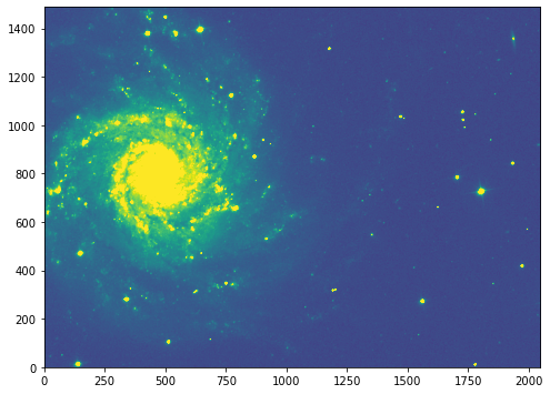
import matplotlib.pyplot as plt
import numpy as np
plt.figure(figsize=(8, 8))
plt.imshow(g_data, vmin=np.min(g_data), vmax=np.mean(g_data)*6 ,origin='lower')
[52]:
<matplotlib.image.AxesImage at 0x7f669a4cb070>
[53]:
from photutils.isophote import EllipseGeometry, Ellipse
x0 = 470.    # center position
y0 = 790.    # center position
sma = 50.   # starting semi-major axis length in pixels
eps = 0.5    # ellipticity
pa = 120. / 180. * np.pi  # position angle

g = EllipseGeometry(x0, y0, sma, eps, pa)
g.find_center(g_data)
ellipse = Ellipse(g_data, geometry=g)
INFO: Found center at x0 = 468.0, y0 = 795.0 [photutils.isophote.geometry]
[54]:
isolist_g = ellipse.fit_image(sclip=3., nclip=3)
[55]:
isolist_g.to_table()
[55]:
| sma | intens | intens_err | ellipticity | ellipticity_err | pa | pa_err | grad | grad_error | grad_rerror | x0 | x0_err | y0 | y0_err | ndata | nflag | niter | stop_code |
|---|---|---|---|---|---|---|---|---|---|---|---|---|---|---|---|---|---|
| deg | deg | ||||||||||||||||
| float64 | float64 | float64 | float64 | float64 | float64 | float64 | float64 | object | object | float64 | float64 | float64 | float64 | int64 | int64 | int64 | int64 |
| 0.0 | 7.036626190437779 | 0.0 | 0.0 | 0.0 | 0.0 | 0.0 | 0.0 | None | None | 467.9179092880445 | 0.0 | 794.383977410454 | 0.0 | 1 | 0 | 0 | 0 |
| 0.5153723524097881 | 6.978559618937684 | 0.008576114152388018 | 0.6694480081838572 | 0.2470076943555362 | 89.90100378535975 | 16.41472690185171 | -0.07912810846330354 | 0.2096983845492498 | 2.6501124394563225 | 467.9179092880445 | 0.06568770710530847 | 794.383977410454 | 0.19267481565129643 | 13 | 0 | 10 | 0 |
| 0.5669095876507669 | 6.960915542591993 | 0.01163991868890307 | 0.6507549612191641 | 0.32495041185875756 | 88.16239100919601 | 21.91215467932307 | -0.07811240659310056 | 0.2524319870075608 | 3.2316503615426613 | 467.9095218688027 | 0.09540039146789599 | 794.4024042095552 | 0.2638530060191995 | 13 | 0 | 15 | 0 |
| 0.6236005464158436 | 6.913445060192853 | 0.014810388687327002 | 0.5214108732949624 | 0.07016612745554274 | 85.75012702336906 | 5.388612235549459 | -0.5741185173579035 | 0.371018363404091 | 0.646240022202244 | 467.8618205519865 | 0.02277388330252793 | 794.4320641048108 | 0.04565890241578605 | 13 | 0 | 14 | 0 |
| 0.685960601057428 | 6.8171311547719675 | 0.018494760884981795 | 0.26213683749883254 | 0.08585925093501036 | 77.48078876555806 | 11.158710663601077 | -0.8196585299530214 | 0.40163216863368667 | 0.48999937651683584 | 467.77047819258416 | 0.03091016946456364 | 794.4473246200079 | 0.03954854930982435 | 13 | 0 | 10 | 0 |
| 0.7545566611631708 | 6.719546613052389 | 0.01917574088778771 | 0.11080964674370897 | 0.0778846547859353 | 55.4251981533052 | 22.027911471709082 | -1.0290186925466056 | 0.36194599542634526 | 0.35173898982398927 | 467.7183786548457 | 0.03124025101747533 | 794.450773580251 | 0.03221662954732579 | 13 | 0 | 10 | 0 |
| 0.8300123272794878 | 6.633136981338138 | 0.017307265730366405 | 0.09490131001622146 | 0.05754882021454632 | 48.05858988632109 | 18.91411388213538 | -1.1654779405711668 | 0.3005154919942702 | 0.25784743025423223 | 467.7044633929275 | 0.025410765475871275 | 794.4679398454274 | 0.025607024778430708 | 13 | 0 | 10 | 0 |
| 0.9130135600074366 | 6.540013643189832 | 0.01761471303679338 | 0.09960426453582245 | 0.05028090800267418 | 47.73863173370245 | 15.730298876801987 | -1.2276012406620995 | 0.27282814174790015 | 0.22224492181251942 | 467.7122031062119 | 0.024533449000052554 | 794.4784320508862 | 0.024707965348026936 | 13 | 0 | 10 | 0 |
| 1.0043149160081803 | 6.4251187693363025 | 0.017538080327585717 | 0.09334886460066218 | 0.043892428927741145 | 49.17325342279127 | 14.601134368666187 | -1.2820088891980004 | 0.2401225159197908 | 0.18730175581700276 | 467.7194249253849 | 0.023440130888446712 | 794.4873080996812 | 0.023669185220263057 | 13 | 0 | 10 | 0 |
| ... | ... | ... | ... | ... | ... | ... | ... | ... | ... | ... | ... | ... | ... | ... | ... | ... | ... |
| 34.15067276825353 | 0.9085946752882448 | 0.008412769157337614 | 0.12329079231438017 | 0.016414555672706884 | 29.237653665651415 | 4.31423584572952 | -0.03681355138113781 | 0.0032104862719673053 | 0.0872093604533972 | 467.70358347485575 | 0.3164089445231044 | 794.5428607809346 | 0.3018385057755577 | 191 | 10 | 10 | 0 |
| 37.56574004507888 | 0.8072671486823538 | 0.005562672982446853 | 0.14516100493855583 | 0.01590797932067167 | 37.957399878882185 | 3.572650807765996 | -0.021913245924082177 | 0.002040055236019722 | 0.09309689870170014 | 467.64177151813936 | 0.33637204448118596 | 795.728062195 | 0.3288987730865621 | 208 | 11 | 50 | 2 |
| 41.32231404958677 | 0.74260716814388 | 0.004606763004680098 | 0.14516100493855583 | 0.01577525741080338 | 37.957399878882185 | 3.351490240800742 | -0.01727367789960801 | 0.0015538063345802758 | 0.08995225820527405 | 465.50780730738984 | 0.35738323885825807 | 795.9432593178165 | 0.34847677228878327 | 239 | 2 | 12 | 0 |
| 45.45454545454545 | 0.6675655260829918 | 0.004019052663012127 | 0.020334419834488394 | 0.014574681190688476 | 174.45886192406857 | 20.83832436329162 | -0.01692291673102629 | 0.0012561202864719793 | 0.07422599227052994 | 468.34887839540784 | 0.3372038338318546 | 792.85323485123 | 0.3336362730177481 | 284 | 0 | 10 | 0 |
| 50.0 | 0.6233688395896823 | 0.0038857790540935753 | 0.07192425672502625 | 0.011473817051920332 | 22.63241566329892 | 4.762788596013085 | -0.017884978187662947 | 0.0010445918855682568 | 0.05840610341302043 | 468.95629351514003 | 0.3039528132731592 | 791.9291057338585 | 0.2931649716067771 | 304 | 0 | 20 | 0 |
| 55.00000000000001 | 0.5527354045615789 | 0.0034136796328234566 | 0.08084739883890796 | 0.012257015176678106 | 57.35934046184081 | 4.536065027367982 | -0.013210050208749756 | 0.0008411819030523203 | 0.0636774190680334 | 468.4830269196794 | 0.34810202647243166 | 793.083407647348 | 0.3561660260924111 | 332 | 1 | 10 | 0 |
| 60.500000000000014 | 0.4641562041293947 | 0.0026370299400790696 | 0.06193362355399344 | 0.038813316025626744 | 25.92245924860833 | 18.478098648962256 | -0.0029653100139409895 | 0.0003206536454149992 | 0.10813494842275884 | 471.3618305005114 | 1.2351977734310622 | 794.4826743505715 | 1.188160798306999 | 390 | 4 | 50 | 2 |
| 66.55000000000003 | 0.4573494796138069 | 0.0027404038997232505 | 0.06193362355399344 | 0.018325023223018527 | 171.46767933571007 | 8.846787668315997 | -0.00592387811267946 | 0.0005752116555117235 | 0.09710052174782957 | 470.078949520937 | 0.6510994486824244 | 794.6751420995071 | 0.6157646319111435 | 397 | 10 | 50 | 2 |
| 73.20500000000004 | 0.41787458466002114 | 0.0026742808876279384 | 0.06193362355399344 | 0.019220655684728024 | 171.46767933571007 | 9.370177531086478 | -0.00446762781459476 | 0.0005017109466401413 | 0.11229918145848268 | 470.078949520937 | 0.7549754474956365 | 794.6751420995071 | 0.7132245446317707 | 433 | 15 | 8 | 5 |
| 80.52550000000005 | 0.38521370470337724 | 0.0025130787847420155 | 0.06193362355399344 | 0.007370023089225932 | 171.46767933571007 | 3.5531305987650277 | -0.0091538954567166 | None | None | 470.078949520937 | 0.31431303411502626 | 794.6751420995071 | 0.30157024802649013 | 489 | 3 | 17 | 5 |
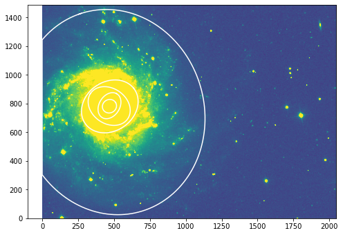
[56]:
fig, ax = plt.subplots(figsize=(8, 8))
plt.imshow(g_data, vmin=np.min(g_data), vmax=np.mean(g_data)*6 ,origin='lower')
#ax.set_title("791 wide filter")
#ax.set_xlim([300, 900])
#ax.set_ylim([700, 1200])

# go to the outermost successfully fitted ellipse at sma=235
isos = []
for sma in [50., 100., 150., 200., 700.]:
    iso = isolist_g.get_closest(sma)
    isos.append(iso)
    x, y, = iso.sampled_coordinates()
    plt.plot(x, y, color='w')

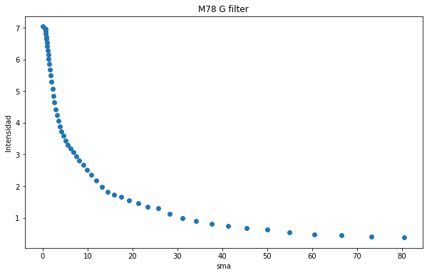
[57]:
plt.figure(figsize=(10, 6))
plt.scatter(isolist_g.sma, isolist_g.intens)
plt.title("M78 G filter")
plt.xlabel('sma')
plt.ylabel('Intensidad')
[57]:
Text(0, 0.5, 'Intensidad')
Ajuste de isofotas en la banda R
[58]:
ellipse = Ellipse(r_data, geometry=g)
isolist_r = ellipse.fit_image(sclip=3., nclip=3)
[59]:
isolist_r.to_table()
[59]:
| sma | intens | intens_err | ellipticity | ellipticity_err | pa | pa_err | grad | grad_error | grad_rerror | x0 | x0_err | y0 | y0_err | ndata | nflag | niter | stop_code |
|---|---|---|---|---|---|---|---|---|---|---|---|---|---|---|---|---|---|
| deg | deg | ||||||||||||||||
| float64 | float64 | float64 | float64 | float64 | float64 | float64 | float64 | object | object | float64 | float64 | float64 | float64 | int64 | int64 | int64 | int64 |
| 0.0 | 15.115861775825355 | 0.0 | 0.0 | 0.0 | 0.0 | 0.0 | 0.0 | None | None | 467.31876720748215 | 0.0 | 782.8102866841725 | 0.0 | 1 | 0 | 0 | 0 |
| 0.5153723524097881 | 14.80854481009532 | 0.03550733923843654 | 0.32807929624430315 | 0.09005891777301354 | 1.6376261808230042 | 9.723721962589002 | -1.8266834486155674 | 1.0760417953786134 | 0.5890685636825248 | 467.31876720748215 | 0.03456715553460349 | 782.8102866841725 | 0.023938229986199124 | 13 | 0 | 10 | 0 |
| 0.5669095876507669 | 14.744955711536875 | 0.039224570005740526 | 0.32754732992918306 | 0.09066629148984201 | 2.1082927874824695 | 9.798557862520317 | -1.8238744749881592 | 1.080699862467699 | 0.5925297367159628 | 467.34896345022264 | 0.03823642987592174 | 782.7916186894681 | 0.02654433985595171 | 13 | 0 | 10 | 0 |
| 0.6236005464158436 | 14.654245875551062 | 0.04417651562546908 | 0.2898650442665084 | 0.07712256784928587 | 2.1082927874824695 | 9.211522229889454 | -2.3138996300117447 | 1.0632070468901071 | 0.45948710700330186 | 467.3848534973449 | 0.03388159760027299 | 782.7568301745149 | 0.024835168866018397 | 13 | 0 | 10 | 0 |
| 0.685960601057428 | 14.411300732930584 | 0.05798061229452439 | 0.10549696928597599 | 0.10292288993304693 | 5.394862425214707 | 30.489754168893068 | -2.6079654833583565 | 1.3055400552356529 | 0.5005971373342216 | 467.39176803364626 | 0.03947324043118913 | 782.6836119474008 | 0.03646434693179429 | 13 | 0 | 10 | 0 |
| 0.7545566611631708 | 14.208786191943034 | 0.06051425737422601 | 0.07479475971806991 | 0.07712400726072463 | 25.417552709318507 | 31.712353702209455 | -3.4192838015490437 | 1.100859644586111 | 0.3219562073459321 | 467.41275311372124 | 0.03121613664354069 | 782.6519681862151 | 0.030304149880922733 | 13 | 0 | 10 | 0 |
| 0.8300123272794878 | 13.923481065183267 | 0.061854413488296706 | 0.04623617842225249 | 0.06723444564375199 | 28.226880911930504 | 44.06783015281843 | -3.7570347313732357 | 0.9949899918254543 | 0.2648338551455911 | 467.4139306822327 | 0.02917443555385493 | 782.6395654472735 | 0.02890583912793097 | 13 | 0 | 10 | 0 |
| 0.9130135600074366 | 13.576650547763618 | 0.05455842505722865 | 0.02556828693214871 | 0.053454722565663165 | 29.229985776638813 | 62.696055514492244 | -3.8711321169825386 | 0.7829759625976392 | 0.20226020165076453 | 467.4156365654137 | 0.025094954453855286 | 782.6414016536859 | 0.025159388406748737 | 13 | 0 | 10 | 0 |
| 1.0043149160081803 | 13.213446815898358 | 0.04572936757899414 | 0.020700524771805628 | 0.04051089878768394 | 29.14358074224163 | 58.541994646833736 | -3.911743273189038 | 0.5844924701081633 | 0.14941994637384712 | 467.4178699098615 | 0.02084172098100342 | 782.6377694289448 | 0.020949201363302142 | 13 | 0 | 10 | 0 |
| ... | ... | ... | ... | ... | ... | ... | ... | ... | ... | ... | ... | ... | ... | ... | ... | ... | ... |
| 305.7954522420732 | 0.2299015931811956 | 0.001049805656182339 | 0.19095531953119518 | 0.005189826786289222 | 127.57366992180178 | 0.8681957482579648 | -0.0015083615289399087 | 4.475764347657719e-05 | 0.0296730211012696 | 480.13750557512543 | 0.8724555385440977 | 782.4864816457109 | 0.9111775803513292 | 1647 | 85 | 10 | 0 |
| 336.37499746628055 | 0.181010503486312 | 0.0008744648830469305 | 0.1683308490779746 | 0.006292500062859602 | 137.28284932652832 | 1.166042036308538 | -0.0009730677078393906 | 3.746726993110771e-05 | 0.038504278406587364 | 483.90980377567126 | 1.1717128433199169 | 783.597410674144 | 1.1579123149338777 | 1880 | 52 | 11 | 0 |
| 370.0124972129086 | 0.15571082955865462 | 0.0008255035794957434 | 0.13805794532331586 | 0.007075611162730078 | 165.17805430019712 | 1.5753762262279287 | -0.0007689894768995144 | 3.148916814676029e-05 | 0.04094876340014605 | 458.65590308954796 | 1.4741959372390454 | 780.1828018707679 | 1.3474643596834859 | 2119 | 46 | 10 | 0 |
| 407.0137469341995 | 0.13239741264163696 | 0.0008435050789037439 | 0.16030507644163722 | 0.006153825994055101 | 175.23289053511024 | 1.183832185580419 | -0.0008041818771965464 | 2.62531979343177e-05 | 0.03264584626781048 | 453.1524762375078 | 1.4571926858382886 | 782.3912846753941 | 1.2687280560778178 | 2257 | 93 | 10 | 0 |
| 447.7151216276195 | 0.08726337479221832 | 0.0006269297915088599 | 0.08462883699479408 | 0.00928665473743837 | 3.5234080075914496 | 3.319459852170743 | -0.0003817893578103019 | 1.9023298963903486e-05 | 0.04982668734667956 | 453.1524762375078 | 2.2674873288501125 | 782.3912846753941 | 2.107069908896665 | 2606 | 96 | 50 | 2 |
| 492.4866337903815 | 0.07803196990125381 | 0.0005686109794194456 | 0.1520600294822607 | 0.0076751334894905624 | 25.00524022412254 | 1.5563953270358457 | -0.0003695511933091765 | 1.6096127382462112e-05 | 0.0435558798723609 | 456.90268633633013 | 2.2220902527134654 | 774.3508531647085 | 1.9177996235025851 | 2509 | 348 | 11 | 0 |
| 541.7352971694197 | 0.06311041079140965 | 0.0005039272563336629 | 0.1520600294822607 | 0.009063698669117553 | 44.526007274994605 | 2.1729338915531096 | -0.00023791141695881884 | 1.4014423267378346e-05 | 0.05890605607129886 | 458.92821671698067 | 2.963895358717135 | 750.5894639461408 | 2.9554782869305645 | 2692 | 451 | 11 | 0 |
| 595.9088268863617 | 0.042310312256476225 | 0.00044575812749738465 | 0.09331850482310948 | 0.014347409524371229 | 71.9766889730873 | 4.493907112347438 | -0.00014574162865291316 | 1.1662918694213359e-05 | 0.0800246216679028 | 486.5237006051657 | 4.743155976582619 | 739.6978242276742 | 4.1886140356823525 | 2986 | 592 | 50 | 2 |
| 655.499709574998 | 0.033515337426171396 | 0.00045660276678671416 | 0.11095321476944284 | 0.011876145386797527 | 105.97288800210559 | 2.961628201424166 | -0.00017150111840922035 | 9.548347123206663e-06 | 0.055675130353513305 | 486.5237006051657 | 4.516828683942675 | 739.6978242276742 | 3.6027776846256727 | 3069 | 828 | 50 | 2 |
| 721.0496805324979 | 0.02227344409526827 | 0.00042808533979924 | 0.11095321476944284 | 0.01252961880425357 | 105.97288800210559 | 3.0404016718398816 | -0.000146315348067615 | 8.39892768526509e-06 | 0.05740291634602674 | 486.5237006051657 | 5.670728370967659 | 739.6978242276742 | 4.0521634358823615 | 3213 | 1074 | 2 | 1 |
[60]:
fig, ax = plt.subplots(figsize=(8, 8))
plt.imshow(r_data, vmin=np.min(g_data), vmax=np.mean(g_data)*6 ,origin='lower')
#ax.set_title("791 wide filter")
#ax.set_xlim([300, 900])
#ax.set_ylim([700, 1200])

# go to the outermost successfully fitted ellipse at sma=235
isos = []
for sma in [50., 100., 150., 200., 700.]:
    iso = isolist_r.get_closest(sma)
    isos.append(iso)
    x, y, = iso.sampled_coordinates()
    plt.plot(x, y, color='w')
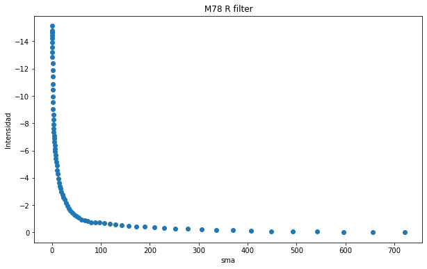
[61]:
plt.figure(figsize=(10, 6))
plt.scatter(isolist_r.sma, -isolist_r.intens)
plt.title("M78 R filter")
plt.xlabel('sma')
plt.ylabel('Intensidad')
plt.gca().invert_yaxis()
Nivel de Ruido de las Imágenes (stdev)
Vamos a obtener el nivel de ruido que tenemos en nuestras imágenes. Para ello nos iremos a una zona donde sepamos que no haya brillo de la galaxia ni de estrellas, es decir una zona donde sea lo mas oscuro posible y solo veamos píxeles de ruido. Una vez que tengamos la zona localizada mediante la desviación cuadrática media stdev podremos ver el nivel de ruido que tenemos en nuestra imagen.
Esto nos servirá para poder distingir señal de ruido a medida que nos vayamos alejando del centro de la galaxia.
[62]:
import matplotlib.pyplot as plt
import numpy as np
plt.figure(figsize=(8, 8))
plt.imshow(g_data[0:100,1900:2000], vmin=np.min(g_data), vmax=np.mean(g_data)*6 ,origin='lower')
[62]:
<matplotlib.image.AxesImage at 0x7f6697404160>
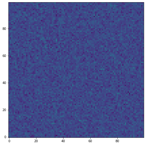
[63]:
g_std = np.std(g_data[0:100,1900:2000])
r_std = np.std(r_data[0:100,1900:2000])

g_std, r_std
[63]:
(0.018639611, 0.031717688)
Escala de píxel en arcsec/pix y en pc/pix de las imágenes.
Mediante los parámetros observados en la cabecera de nuestras imágenes calculamos el diámetro angular como: $ D = \sqrt{CD1\_1^2 + CD2\_1^2} *3600 $
[64]:
D_arc = np.sqrt(g_header['CD1_1']**2+g_header['CD2_1']**2)*3600 #arcsec/pix
D_arc
[64]:
0.39595593301525844
Para obtener el valor de parsec por pixel deberemos hacer la transformación del diámetro angular en arcoseg/pixel a radianes/pixel y este multiplicarlo por la distancia a la galaxia. Para el valor de la distancia a la galaxia hemos tomado como referencia el método SNII optical en la banda B, \(d = 7.2 Mpc\).
[65]:
D_pc = (D_arc/3600)*(np.pi/180)*(7.2*10**6)
D_pc #pc/pixel
[65]:
13.821469447844759
Calibración del flujo
Para calcular el brillo superficial que tiene nuestra galaxia medido a través de las imágenes recogidas, tenemos que tener en cuenta que la medida de intensidad de las imágenes esta en nanomaggies. Podemos pasar de nanomaggies a magnitudes usando la siguiente formula:
y por lo tanto podemos calcular el brillo superficial mediante el uso de la resolución angular.
[66]:
def mu(nanomaggies, D):
    return 22.5-2.5*np.log10(nanomaggies/D**2)
Para calcular la magnitud límite vamos a considerar que el brillo mas bajo medible es 3 veces el ruido de fondo que tengamos en nuestra imagen.
[67]:
mag_lim_g = mu(3*g_std, D_arc) #mag/arcsec**2
mag_lim_r = mu(3*r_std, D_arc) #mag/arcsec**2
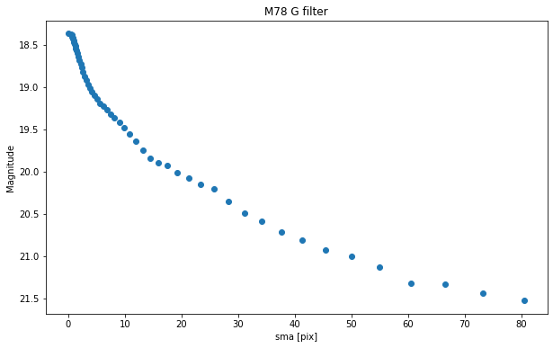
Ajustar el perfil de brillo del disco y obtener la longitud de escala
Banda G
[68]:
plt.figure(figsize=(10, 6))
plt.scatter(isolist_g.sma, mu(isolist_g.intens, D_arc))
plt.title("M78 G filter")
plt.xlabel('sma [pix]')
plt.ylabel('Magnitude')
plt.gca().invert_yaxis()
[69]:
np.where(isolist_g.sma <=90)
[69]:
(array([ 0,  1,  2,  3,  4,  5,  6,  7,  8,  9, 10, 11, 12, 13, 14, 15, 16,
        17, 18, 19, 20, 21, 22, 23, 24, 25, 26, 27, 28, 29, 30, 31, 32, 33,
        34, 35, 36, 37, 38, 39, 40, 41, 42, 43, 44, 45, 46, 47, 48, 49, 50,
        51, 52, 53, 54]),)
[70]:
plt.figure(figsize=(10, 6))
plt.scatter(isolist_g.sma[55:], mu(isolist_g.intens[55:], D_arc), label= 'Perfil de brillo')
plt.title("M78 G filter")
plt.xlabel('sma [pix]')
plt.ylabel('Magnitude')
plt.gca().invert_yaxis()
plt.axhline(y=mag_lim_g, label='Magnitud límite')
plt.legend()
[70]:
<matplotlib.legend.Legend at 0x7f6697090ee0>
[71]:
np.where(isolist_g.sma <=500)
[71]:
(array([ 0,  1,  2,  3,  4,  5,  6,  7,  8,  9, 10, 11, 12, 13, 14, 15, 16,
        17, 18, 19, 20, 21, 22, 23, 24, 25, 26, 27, 28, 29, 30, 31, 32, 33,
        34, 35, 36, 37, 38, 39, 40, 41, 42, 43, 44, 45, 46, 47, 48, 49, 50,
        51, 52, 53, 54]),)
[72]:
plt.figure(figsize=(10, 6))
plt.scatter(isolist_g.sma[55:73], mu(isolist_g.intens[55:73], D_arc), label= 'Perfil de brillo')
plt.title("M78 g filter")
plt.xlabel('sma')
plt.ylabel('Magnitude')
plt.gca().invert_yaxis()
plt.legend()
[72]:
<matplotlib.legend.Legend at 0x7f669705dc70>
Ajuste lineal en la banda G
[73]:
import numpy as np
import matplotlib.pyplot as plt
from astropy.modeling import models, fitting

# Definimos el modelo lineal
line_orig = models.Linear1D(slope=1.0, intercept=0.5)
fit = fitting.LinearLSQFitter()
# Inicializamos el modelo lineal
line_init = models.Linear1D()

# Ajuste de los datos
fitted_line_g = fit(line_init, isolist_g.sma[55:73], mu(isolist_g.intens[55:73], D_arc))
/home/zerjillo/anaconda3/envs/cursoAstronomia2/lib/python3.8/site-packages/astropy/modeling/fitting.py:828: RuntimeWarning: invalid value encountered in true_divide
  lacoef /= scl[:, np.newaxis] if scl.ndim < rhs.ndim else scl
[74]:
fitted_line_g
[74]:
<Linear1D(slope=nan, intercept=nan)>
[75]:
plt.figure(figsize=(10, 6))
plt.scatter(isolist_g.sma[55:73], mu(isolist_g.intens[55:73], D_arc), label= 'Perfil de brillo')
plt.plot(x, fitted_line_g(x), 'k-', label='Ajuste lineal')
plt.title("M78 g filter")
plt.xlabel('sma')
plt.ylabel('Magnitude')
plt.xlim(80, 500)
plt.gca().invert_yaxis()
plt.legend()
[75]:
<matplotlib.legend.Legend at 0x7f6696f9e3d0>
La longitud de escala es el radio en el que la galaxia es un factor e (~2,7) menos brillante que en su centro. Debido a la diversidad de formas y tamaños de las galaxias, no todos los discos galácticos siguen esta sencilla forma exponencial en sus perfiles de brillo.
En galaxias espirales el perfil de brillo superficial en el disco se modeliza como:
donde \(\mu_0\) es el brillo de la superficial central y \(H_r\) la longitud de la escala del disco.
Como hemos obtenido la representacion de µ frente a R y hemos ajustado la recta, podemos obtener \(H_R\) mediante la pendiente:
Con un error asociado de :
[76]:
fitted_line_g.slope[0] # pendiente
[76]:
nan
[77]:
1.086/fitted_line_g.slope[0] #pixeles
[77]:
nan
[78]:
1.086/(fitted_line_g.slope[0]*D_arc) #arcsec
[78]:
nan
[79]:
Hr_g = 1.086/fitted_line_g.slope[0]*D_pc #pc
Banda r
[80]:
plt.figure(figsize=(10, 6))
plt.scatter(isolist_r.sma, mu(isolist_r.intens, D_arc))
plt.title("M78 r filter")
plt.xlabel('sma**1/4')
plt.ylabel('Magnitude')
plt.gca().invert_yaxis()
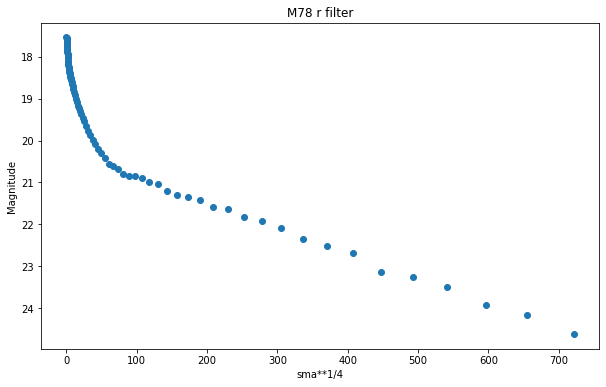
[81]:
np.where(isolist_r.sma <=70)
[81]:
(array([ 0,  1,  2,  3,  4,  5,  6,  7,  8,  9, 10, 11, 12, 13, 14, 15, 16,
        17, 18, 19, 20, 21, 22, 23, 24, 25, 26, 27, 28, 29, 30, 31, 32, 33,
        34, 35, 36, 37, 38, 39, 40, 41, 42, 43, 44, 45, 46, 47, 48, 49, 50,
        51, 52]),)
[82]:
plt.figure(figsize=(10, 6))
plt.scatter(isolist_r.sma[52:], mu(isolist_r.intens[52:], D_arc), label= 'Perfil de brillo')
plt.title("M78 r filter")
plt.xlabel('sma [pix]')
plt.ylabel('Magnitude')
plt.gca().invert_yaxis()
plt.axhline(y=mag_lim_r, label='Magnitud límite')
plt.legend()
[82]:
<matplotlib.legend.Legend at 0x7f66970b70a0>
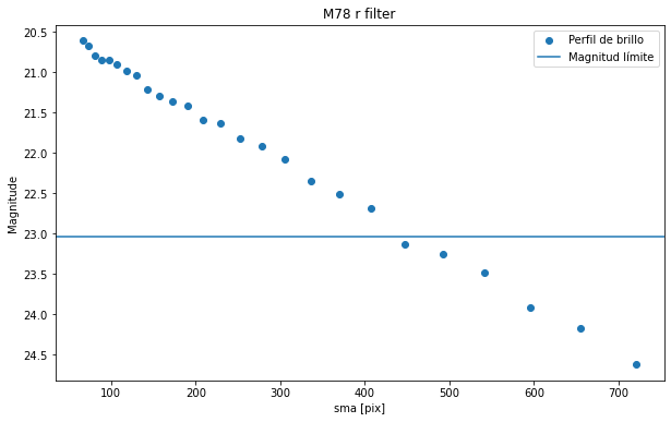
[83]:
np.where(isolist_r.sma <=450)
[83]:
(array([ 0,  1,  2,  3,  4,  5,  6,  7,  8,  9, 10, 11, 12, 13, 14, 15, 16,
        17, 18, 19, 20, 21, 22, 23, 24, 25, 26, 27, 28, 29, 30, 31, 32, 33,
        34, 35, 36, 37, 38, 39, 40, 41, 42, 43, 44, 45, 46, 47, 48, 49, 50,
        51, 52, 53, 54, 55, 56, 57, 58, 59, 60, 61, 62, 63, 64, 65, 66, 67,
        68, 69, 70, 71, 72]),)
[84]:
plt.figure(figsize=(10, 6))
plt.scatter(isolist_g.sma[55:72], mu(isolist_g.intens[55:72], D_arc), label= 'Perfil de brillo')
plt.title("M78 r filter")
plt.xlabel('sma')
plt.ylabel('Magnitude')
plt.gca().invert_yaxis()
plt.legend()
[84]:
<matplotlib.legend.Legend at 0x7f669a9ca340>
Ajuste lineal en la banda r
[85]:
import numpy as np
import matplotlib.pyplot as plt
from astropy.modeling import models, fitting

# Definimos el modelo lineal
line_orig = models.Linear1D(slope=1.0, intercept=0.5)

# Inicializamos el modelo lineal
line_init = models.Linear1D()

# Ajuste de los datos
fitted_line_r = fit(line_init, isolist_r.sma[52:72], mu(isolist_r.intens[52:72], D_arc))
[86]:
fitted_line_r
[86]:
<Linear1D(slope=0.00599491, intercept=20.28690473)>
[87]:
plt.figure(figsize=(10, 6))
plt.scatter(isolist_r.sma[55:73], mu(isolist_r.intens[55:73], D_arc), label= 'Perfil de brillo')
plt.plot(x, fitted_line_r(x), 'k-', label='Ajuste lineal')
plt.title("M78 r filter")
plt.xlabel('sma')
plt.ylabel('Magnitude')
plt.xlim(80, 500)
plt.gca().invert_yaxis()
plt.legend()
[87]:
<matplotlib.legend.Legend at 0x7f669ab69070>
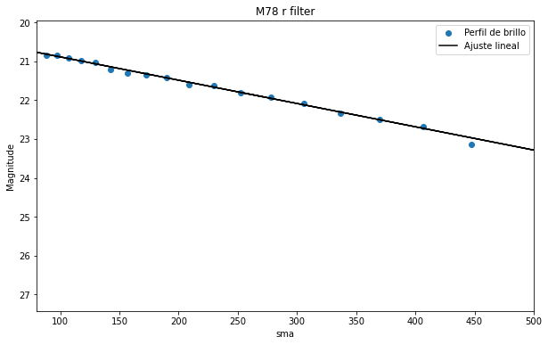
Longitudes de escala
[88]:
fitted_line_r.slope[0]
[88]:
0.0059949075577498375
[89]:
1.086/fitted_line_r.slope[0] #pixeles
[89]:
181.1537525038377
[90]:
1.086/fitted_line_r.slope[0]*D_arc #arcsec
[90]:
71.72890309187227
[91]:
Hr_r = 1.086/fitted_line_r.slope[0]*D_pc #pc
Banda |
H_r[arcsec] |
H_r[pc] |
|---|---|---|
g |
72.06 |
2789.89 |
r |
79.92 |
2515.59 |
[92]:
Hr_g, Hr_r
[92]:
(nan, 2503.8110555942235)
En este articulo podemos encontrar valores aproximados a los que hemos obtenido nosotros, teniendo en cuenta que ellos han cogido una distancia a la galaxia de \(10.4 \: Mpc\):
Banda |
H_r[pc] |
|---|---|
U |
4.26 |
B |
3.44 |
V |
3.27 |
R |
3.29 |
I |
3.31 |
[93]:
D_pc = (D_arc/3600)*(np.pi/180)*(10.4*10**6)
[94]:
Hr_g = 1.086/fitted_line_g.slope[0]*D_pc #pc
Hr_r = 1.086/fitted_line_r.slope[0]*D_pc #pc
Hr_g, Hr_r
[94]:
(nan, 3616.6159691916564)
Diagramas g-r
Como hemos calculado el brillo superficial de la galaxia podemos calcular el color simplemente restando los dos brillos superficiales µG y µR, ya que
[95]:
g_data_mag = 22.5-2.5 * np.log10(g_data/D_arc**2)
r_data_mag = 22.5-2.5 * np.log10(r_data/D_arc**2)
<ipython-input-95-dfe2658c2d03>:1: RuntimeWarning: invalid value encountered in log10
  g_data_mag = 22.5-2.5 * np.log10(g_data/D_arc**2)
<ipython-input-95-dfe2658c2d03>:2: RuntimeWarning: invalid value encountered in log10
  r_data_mag = 22.5-2.5 * np.log10(r_data/D_arc**2)
[96]:
g_r = g_data_mag - r_data_mag
[97]:
plt.figure(figsize=(10, 6))

plt.imshow(g_r, cmap='gray')
[97]:
<matplotlib.image.AxesImage at 0x7f66a1b13970>
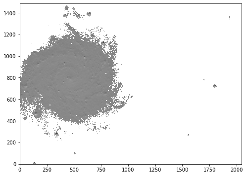
[98]:
plt.figure(figsize=(10, 6))
plt.plot(range(len(g_r[795,468:1000])), g_r[795,468:1000], 'k-', label='Ajuste lineal')
plt.legend()
[98]:
<matplotlib.legend.Legend at 0x7f669abf7fd0>
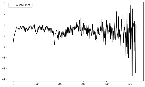
[99]:
g_r = mu(isolist_g.intens[:73],D_arc) - mu(isolist_r.intens[:73],D_arc)
---------------------------------------------------------------------------
ValueError                                Traceback (most recent call last)
Cell In[99], line 1
----> 1 g_r = mu(isolist_g.intens[:73],D_arc) - mu(isolist_r.intens[:73],D_arc)

ValueError: operands could not be broadcast together with shapes (55,) (73,)
[100]:
plt.figure(figsize=(10, 6))
plt.plot(isolist_r.sma[:73], g_r, 'k-', label='Ajuste lineal')
plt.xlabel('sma')
plt.ylabel('g-r')
plt.legend()
plt.show()
---------------------------------------------------------------------------
ValueError                                Traceback (most recent call last)
Cell In[100], line 2
      1 plt.figure(figsize=(10, 6))
----> 2 plt.plot(isolist_r.sma[:73], g_r, 'k-', label='Ajuste lineal')
      3 plt.xlabel('sma')
      4 plt.ylabel('g-r')

File ~/anaconda3/envs/cursoAstronomia2/lib/python3.8/site-packages/matplotlib/pyplot.py:2812, in plot(scalex, scaley, data, *args, **kwargs)
   2810 @_copy_docstring_and_deprecators(Axes.plot)
   2811 def plot(*args, scalex=True, scaley=True, data=None, **kwargs):
-> 2812     return gca().plot(
   2813         *args, scalex=scalex, scaley=scaley,
   2814         **({"data": data} if data is not None else {}), **kwargs)

File ~/anaconda3/envs/cursoAstronomia2/lib/python3.8/site-packages/matplotlib/axes/_axes.py:1688, in Axes.plot(self, scalex, scaley, data, *args, **kwargs)
   1445 """
   1446 Plot y versus x as lines and/or markers.
   1447
   (...)
   1685 (``'green'``) or hex strings (``'#008000'``).
   1686 """
   1687 kwargs = cbook.normalize_kwargs(kwargs, mlines.Line2D)
-> 1688 lines = [*self._get_lines(*args, data=data, **kwargs)]
   1689 for line in lines:
   1690     self.add_line(line)

File ~/anaconda3/envs/cursoAstronomia2/lib/python3.8/site-packages/matplotlib/axes/_base.py:311, in _process_plot_var_args.__call__(self, data, *args, **kwargs)
    309     this += args[0],
    310     args = args[1:]
--> 311 yield from self._plot_args(
    312     this, kwargs, ambiguous_fmt_datakey=ambiguous_fmt_datakey)

File ~/anaconda3/envs/cursoAstronomia2/lib/python3.8/site-packages/matplotlib/axes/_base.py:504, in _process_plot_var_args._plot_args(self, tup, kwargs, return_kwargs, ambiguous_fmt_datakey)
    501     self.axes.yaxis.update_units(y)
    503 if x.shape[0] != y.shape[0]:
--> 504     raise ValueError(f"x and y must have same first dimension, but "
    505                      f"have shapes {x.shape} and {y.shape}")
    506 if x.ndim > 2 or y.ndim > 2:
    507     raise ValueError(f"x and y can be no greater than 2D, but have "
    508                      f"shapes {x.shape} and {y.shape}")

ValueError: x and y must have same first dimension, but have shapes (73,) and (1489, 2048)
Podemos ver un decaimiento en el índice de color hacia el rojo a medida que nos alejamos del radio pero tenemos zonas donde el indice de color se desplaza hacia el azul que se debe a las diferentes edades de las poblaciones estelares del disco, el cual está dominado en las partes externas por estrellas más jóvenes.