E: Introducción al trabajo con imágenes astronómicas (`FITS`)¶

El tipo de archivo de imágenes que usaremos es el formato FITS (Flexible Image Transport System) (documentación sobre este formato) ya que es el estándar que se usa en datos astronómicos. En este tipo de archivo almacenaremos los datos recogidos por el sensor de la cámara, así como los metadatos.

Instalar e importar la biblioteca `astropy`¶

Astropy (web de Astropy) es una biblioteca que pretende aunar todos los paquetes de interés para la astronomía de tal manera que sea fácil importarlos e interaccionar con ellos. El método recomendado de instalación, tal y como pone la documentación es utilizando el siguiente comando de Anaconda:

> conda install astropy

Para manejar imágenes FITS usaremos el modulo fits web de Astropy:

[1]:

from astropy.io import fits

Localizar el directorio y fichero de la imagen que queremos abrir.

[2]:

imagenFits = 'imagenes/tarantula/h.fts'

Declaramos una variable para asignar el archivo .fits y lo abrimos con fits.open()

[3]:

hdul = fits.open(imagenFits)

La función open devuelve un objeto llamado HDUL (lista de HDUs) que es una colección de objetos HDU. Una HDU (Header Data Unit) es la componente de más alto nivel de la estructura de archivos FITS, que consiste en un encabezado y en una matriz o tabla de datos.

Una vez abierta la imagen, hdul[0] es la HDU principal, hdul[1] es la primera extensión HDU, etc.

[4]:

hdul.info()

Filename: imagenes/tarantula/h.fts
No.    Name      Ver    Type      Cards   Dimensions   Format
  0  PRIMARY       1 PrimaryHDU     124   (4096, 4096)   int16 (rescales to uint16)

Como vemos nuestra imagen solo tiene una componente, por lo tanto hdul[0] será nuestra imagen.

[5]:

imagen = hdul[0]

[6]:

type(imagen)

[6]:

astropy.io.fits.hdu.image.PrimaryHDU

La cabecera de un fichero `FITS`¶

Cada elemento de un HDUL es un objeto HDU con los atributos .header y .data, que se pueden usar para acceder a los datos y metadatos (cabecera, header) de la HDU.

Para aquellos que no están familiarizados con los encabezados FITS, consisten en una lista que contiene palabras claves(keys), un valor y un comentario. Tanto la palabra clave como el comentario deben ser cadenas, mientras que el valor puede ser una cadena, un número entero, un número float, un número complejo o booleano. Las palabras clave suelen ser únicas dentro de un encabezado, excepto en algunos casos especiales.

[7]:

header_imagen = imagen.header
header_imagen

[7]:

SIMPLE  =                    T
BITPIX  =                   16 /8 unsigned int, 16 & 32 int, -32 & -64 real
NAXIS   =                    2 /number of axes
NAXIS1  =                 4096 /fastest changing axis
NAXIS2  =                 4096 /next to fastest changing axis
BSCALE  =   1.0000000000000000 /physical = BZERO + BSCALE*array_value
BZERO   =   32768.000000000000 /physical = BZERO + BSCALE*array_value
DATE-OBS= '2020-02-08T03:06:15' / [ISO 8601] UTC date/time of exposure start
EXPTIME =   3.00000000000E+002 / [sec] Duration of exposure
EXPOSURE=   3.00000000000E+002 / [sec] Duration of exposure
SET-TEMP=  -30.000000000000000 /CCD temperature setpoint in C
CCD-TEMP=  -30.000000000000000 /CCD temperature at start of exposure in C
XPIXSZ  =   9.0000000000000000 /Pixel Width in microns (after binning)
YPIXSZ  =   9.0000000000000000 /Pixel Height in microns (after binning)
XBINNING=                    1 / Binning level along the X-axis
YBINNING=                    1 / Binning level along the Y-axis
XORGSUBF=                    0 /Subframe X position in binned pixels
YORGSUBF=                    0 /Subframe Y position in binned pixels
READOUTM= '1 MHz   ' /          Readout mode of image
FILTER  = 'H-alpha '           / Filter name
IMAGETYP= 'Light Frame' /       Type of image
TRAKTIME=   5.0000000000000000 /Exposure time used for autoguiding
FOCALLEN=               1936.1 / Focal length of telescope in mm
APTDIA  =   500.00000000000000 /Aperture diameter of telescope in mm
APTAREA =   178678.08714509010 /Aperture area of telescope in mm^2
SBSTDVER= 'SBFITSEXT Version 1.0' /Version of SBFITSEXT standard in effect
SWCREATE= 'MaxIm DL Version 6.09 160704 03UA3' /Name of software
SWSERIAL= '03UA3-CEEN7-J299Y-94VNY-U13XJ-E0' /Software serial number
SITELAT = '-30 28 15' /         Latitude of the imaging location
SITELONG= '-70 45 54' /         Longitude of the imaging location
JD      =   2458887.6293402780 /Julian Date at start of exposure
OBJECT  = 'NGC2070 '           / Target object name
TELESCOP= 'ACP->Astrooptik'    / Telescope name
INSTRUME= 'FLI     '           / Detector instrument name
OBSERVER= 'Telescope3'         / Observer name
NOTES   = '        '
FLIPSTAT= '        '
CSTRETCH= 'Medium  ' /          Initial display stretch mode
CBLACK  =                 1153 /Initial display black level in ADUs
CWHITE  =                 1809 /Initial display white level in ADUs
PEDESTAL=                    0 /Correction to add for zero-based ADU
SWOWNER = 'Ivan Rubtsov' /      Licensed owner of software
JD-OBS  =      2458887.6293403
HJD-OBS =      2458887.6290039
BJD-OBS =      2458887.6298332
OBJCTAZ =             194.8251
AZIMUTH =             194.8251
OBJCTALT=              47.7458
ALTITUDE=              47.7458
OBJCTHA = '01 56 39.40'
HA      = '01 56 39.40'
PIERSIDE= 'EAST    '
READMODE= '1 MHz   '
AMBTEMP =                   17
HISTORY File was processed by PinPoint 6.1.3 at 2020-02-08T03:11:57
DATE    = '08/02/20'           / [old format] UTC date of exposure start
TIME-OBS= '03:06:15'           / [old format] UTC time of exposure start
UT      = '03:06:15'           / [old format] UTC time of exposure start
TIMESYS = 'UTC     '           / Default time system
RADECSYS= 'FK5     '           / Equatorial coordinate system
AIRMASS =   1.35694060364E+000 / Airmass (multiple of zenithal airmass)
ST      = '07 34 00.40'        / Local apparent sidereal time of exp. start
LAT-OBS =  -3.04711111111E+001 / [deg +N WGS84] Geodetic latitude
LONG-OBS=  -7.07647222222E+001 / [deg +E WGS84] Geodetic longitude
ALT-OBS =   1.58000000000E+003 / [metres] Altitude above mean sea level
OBSERVAT= 'CHILESCOPE'         / Observatory name
RA      = '05 37 21.00'        / [hms J2000] Target right ascension
OBJCTRA = '05 37 21.00'        / [hms J2000] Target right ascension
DEC     = '-69 19 31.0'        / [dms +N J2000] Target declination
OBJCTDEC= '-69 19 31.0'        / [dms +N J2000] Target declination
HISTORY File was processed by PinPoint 6.1.3 at 2020-02-08T03:12:20
FWHM    =   3.78270782232E+000 / [pixels] Mean Full-Width-Half-Max of image star
ZMAG    =   1.76985452953E+001 / Mag zero point for 1 sec exposure
EQUINOX =               2000.0 / Equatorial coordinates are J2000
EPOCH   =               2000.0 / (incorrect but needed by old programs)
PA      =   8.92717748132E+001 / [deg, 0-360 CCW] Position angle of plate
CTYPE1  = 'RA---TAN'           / X-axis coordinate type
CRVAL1  =   8.43359148996E+001 / X-axis coordinate value
CRPIX1  =   2.04800000000E+003 / X-axis reference pixel
CDELT1  =  -2.66001231144E-004 / [deg/pixel] X-axis plate scale
CROTA1  =  -8.92717748132E+001 / [deg] Roll angle wrt X-axis
CTYPE2  = 'DEC--TAN'           / Y-axis coordinate type
CRVAL2  =  -6.93257259717E+001 / Y-axis coordinate value
CRPIX2  =   2.04800000000E+003 / Y-axis reference pixel
CDELT2  =  -2.65964401525E-004 / [deg/pixel] Y-Axis Plate scale
CROTA2  =  -8.92717748132E+001 / [deg] Roll angle wrt Y-axis
CD1_1   =  -3.38076526016E-006 / Change in RA---TAN along X-Axis
CD1_2   =  -2.65942919570E-004 / Change in RA---TAN along Y-Axis
CD2_1   =   2.65979746215E-004 / Change in DEC--TAN along X-Axis
CD2_2   =  -3.38029717098E-006 / Change in DEC--TAN along Y-Axis
TR1_0   =   2.04799977556E+003 / [private] X-axis distortion coefficients
TR1_1   =   4.09600822918E+003
TR1_2   =  -9.27752874369E-001
TR1_3   =   9.17573349534E-002
TR1_4   =  -7.71299189613E-001
TR1_5   =  -2.34136010643E-001
TR1_6   =  -7.32598138490E+001
TR1_7   =   7.20318152719E-001
TR1_8   =  -7.24302799606E+001
TR1_9   =  -2.13102413908E+000
TR1_10  =   1.02429158182E+000
TR1_11  =  -2.18328671392E+000
TR1_12  =   1.25055870525E+000
TR1_13  =   2.62261766608E+000
TR1_14  =   3.90939746288E+000
TR2_0   =   2.04799999900E+003 / [private] Y-axis distortion coefficients
TR2_1   =   4.27111011392E-003
TR2_2   =   4.09599166348E+003
TR2_3   =   5.38729172019E-001
TR2_4   =   8.86546806393E-001
TR2_5   =  -1.39307809623E+000
TR2_6   =   1.60951857270E+000
TR2_7   =  -7.04696501405E+001
TR2_8   =  -8.76500526243E-001
TR2_9   =  -7.11088676599E+001
TR2_10  =  -3.52621540448E+000
TR2_11  =  -1.34522966608E+000
TR2_12  =  -8.54364594815E-001
TR2_13  =  -3.65722689398E+000
TR2_14  =   4.72692785031E+000
HISTORY WCS added by PinPoint 6.1.3 at 2020-02-08T03:12:21
HISTORY   Matched 209 stars from the Gray GSC-ACT Catalog
HISTORY   Average residual was 0.29 arc-seconds
PLTSOLVD=                    T / Plate has been solved by PinPoint

Para obtener el valor asociado con una palabra clave, operamos como si fuera un diccionario.

Aunque los nombres de las palabras clave siempre están en mayúsculas dentro del archivo FITS, una palabra clave con astropy no distingue entre mayúsculas y minúsculas para comodidad del usuario ;)

Si el nombre de la palabra clave especificada no existe, generará una KeyErrorexcepción.

[8]:

print(header_imagen['RA'])
print(header_imagen['ra'])

05 37 21.00
05 37 21.00

A los valores de las claves se puede acceder a través de la posición en la lista pero esto no resulta muy útil ya que cada cabecera puede estar distribuida de una forma diferente:

[9]:

print(header_imagen[4])    # Mejor no acceder de esta manera

Los valores de estas palabras clave pueden tener asociados comentarios que podemos leer con el atributo .comments['']

[10]:

header_imagen.comments['RA']

[10]:

'[hms J2000] Target right ascension'

Para actualizar el valor de una clave o para generar una nueva nos basta con el método .set() o al igual que en un diccionario sobrescribir o crear la clave que queramos. ¡Ojo! No estamos grabando los cambios en la cabecera en el fichero de disco, sino en la imagen que tenemos cargada en memoria. Más adelante veremos como guardar una imagen modificada en el disco.

[11]:

print(header_imagen['observer'])
header_imagen.set('observer', 'SAG')
print(header_imagen['observer'])
header_imagen['observer'] = 'Javier'
print(header_imagen['observer'])

Telescope3
SAG
Javier

Podemos también actualizar tanto el valor como el comentario asociado a una palabra clave asignándole una tupla:

[12]:

header_imagen['Observer'] = ('SAG', 'El telescopio es un ASA')
print(f"Valor: {header_imagen['Observer']}")
print(f"Comentario: {header_imagen.comments['Observer']}")

Valor: SAG
Comentario: El telescopio es un ASA

Podemos acceder a un historial y a los comentarios de la imagen:

[13]:

print(header_imagen['history'])
header_imagen['comment'] = 'estos son los comentarios de mi imagen'
print('')
print(header_imagen['comment'])

File was processed by PinPoint 6.1.3 at 2020-02-08T03:11:57
File was processed by PinPoint 6.1.3 at 2020-02-08T03:12:20
WCS added by PinPoint 6.1.3 at 2020-02-08T03:12:21
  Matched 209 stars from the Gray GSC-ACT Catalog
  Average residual was 0.29 arc-seconds

estos son los comentarios de mi imagen

Si vamos a realizar modificiaciones en nuestro fichero es buena práctica añadir en la cabecera información sobre el procesado que se ha aplicado. Por ejemplo podemos indicar que se han aplicado flats o darks, etc.

Podemos obtener una lista con todas las claves que tiene nuestro header con el método .keys()

[14]:

list(header_imagen.keys())

[14]:

['SIMPLE',
 'BITPIX',
 'NAXIS',
 'NAXIS1',
 'NAXIS2',
 'BSCALE',
 'BZERO',
 'DATE-OBS',
 'EXPTIME',
 'EXPOSURE',
 'SET-TEMP',
 'CCD-TEMP',
 'XPIXSZ',
 'YPIXSZ',
 'XBINNING',
 'YBINNING',
 'XORGSUBF',
 'YORGSUBF',
 'READOUTM',
 'FILTER',
 'IMAGETYP',
 'TRAKTIME',
 'FOCALLEN',
 'APTDIA',
 'APTAREA',
 'SBSTDVER',
 'SWCREATE',
 'SWSERIAL',
 'SITELAT',
 'SITELONG',
 'JD',
 'OBJECT',
 'TELESCOP',
 'INSTRUME',
 'OBSERVER',
 'NOTES',
 'FLIPSTAT',
 'CSTRETCH',
 'CBLACK',
 'CWHITE',
 'PEDESTAL',
 'SWOWNER',
 'JD-OBS',
 'HJD-OBS',
 'BJD-OBS',
 'OBJCTAZ',
 'AZIMUTH',
 'OBJCTALT',
 'ALTITUDE',
 'OBJCTHA',
 'HA',
 'PIERSIDE',
 'READMODE',
 'AMBTEMP',
 'HISTORY',
 'DATE',
 'TIME-OBS',
 'UT',
 'TIMESYS',
 'RADECSYS',
 'AIRMASS',
 'ST',
 'LAT-OBS',
 'LONG-OBS',
 'ALT-OBS',
 'OBSERVAT',
 'RA',
 'OBJCTRA',
 'DEC',
 'OBJCTDEC',
 'HISTORY',
 'FWHM',
 'ZMAG',
 'EQUINOX',
 'EPOCH',
 'PA',
 'CTYPE1',
 'CRVAL1',
 'CRPIX1',
 'CDELT1',
 'CROTA1',
 'CTYPE2',
 'CRVAL2',
 'CRPIX2',
 'CDELT2',
 'CROTA2',
 'CD1_1',
 'CD1_2',
 'CD2_1',
 'CD2_2',
 'TR1_0',
 'TR1_1',
 'TR1_2',
 'TR1_3',
 'TR1_4',
 'TR1_5',
 'TR1_6',
 'TR1_7',
 'TR1_8',
 'TR1_9',
 'TR1_10',
 'TR1_11',
 'TR1_12',
 'TR1_13',
 'TR1_14',
 'TR2_0',
 'TR2_1',
 'TR2_2',
 'TR2_3',
 'TR2_4',
 'TR2_5',
 'TR2_6',
 'TR2_7',
 'TR2_8',
 'TR2_9',
 'TR2_10',
 'TR2_11',
 'TR2_12',
 'TR2_13',
 'TR2_14',
 'HISTORY',
 'HISTORY',
 'HISTORY',
 'PLTSOLVD',
 'COMMENT']

Los datos de la imagen `FITS`¶

Si los datos HDU son los de una imagen, el atributo de datos del objeto HDU devolverá un ndarray de numpy (matrices numéricas). La biblioteca numpyestá especializada en operar sobre matrices de manera muy eficiente como iremos viendo.

[15]:

data_imagen = imagen.data
type(data_imagen)

[15]:

numpy.ndarray

El objeto devuelto ndarray tiene muchos atributos y métodos para obtener información sobre la matriz, por ejemplo:

[16]:

data_imagen.shape

[16]:

(4096, 4096)

Los objetos ndarrayse asemejan mucho a las listas, con lo que podemos podemos dividirlos, verlos y realizar operaciones matemáticas en ellos. Por ejemplo, para ver el valor de píxel en x=20, y=20:

[17]:

data_imagen[19,19]

[17]:

Recuerda que en Python la primera posición de una lista tiene un índice 0 (empieza a contar en el 0). Además, una particularidad para las imágenes 2D es que el eje X es el segundo índice: Si queremos recortar los valores de los píxeles entre \(x \in [11,20]\) e \(y \in [31, 40]\) (suponiendo que nosotros empezamos a contar por 1) podríamos hacerlo así:

[18]:

data_imagen[30:40, 10:20] #[y:x]

[18]:

array([[1118, 1151, 1146, 1119, 1133, 1126, 1144, 1148, 1150, 1130],
       [1148, 1119, 1133, 1123, 1134, 1140, 1103, 1147, 1134, 1127],
       [1133, 1142, 1124, 1120, 1136, 1124, 1136, 1147, 1116, 1136],
       [1134, 1133, 1135, 1140, 1143, 1151, 1140, 1138, 1162, 1159],
       [1145, 1133, 1147, 1133, 1144, 1141, 1159, 1119, 1143, 1139],
       [1138, 1135, 1128, 1136, 1101, 1115, 1150, 1144, 1105, 1120],
       [1111, 1153, 1146, 1121, 1146, 1119, 1133, 1133, 1115, 1128],
       [1126, 1148, 1134, 1123, 1129, 1128, 1144, 1131, 1139, 1148],
       [1131, 1114, 1128, 1127, 1124, 1130, 1114, 1127, 1159, 1157],
       [1142, 1123, 1146, 1125, 1136, 1122, 1137, 1140, 1117, 1121]],
      dtype=uint16)

Graficando imágenes `FITS`¶

Para mostrar la imagen usaremos la biblioteca Matplotlib (enlace a su documentación):

[19]:

import matplotlib.pyplot as plt
import numpy as np

[20]:

plt.imshow(data_imagen)

[20]:

<matplotlib.image.AxesImage at 0x7f7f82256730>

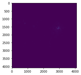
_images/E-1-introduccion_imagenes_astronomicas_41_1.png

La imagen resultante es un poco pequeña y los ejes de coordenadas están dispuestos de una manera poco intuitiva. Podemos mejorar nuestra imagen ajustando algunos parámetros de la gráfica:

[21]:

plt.figure(figsize=(10,10))
plt.imshow(data_imagen, origin='lower')

[21]:

<matplotlib.image.AxesImage at 0x7f7f780dd040>

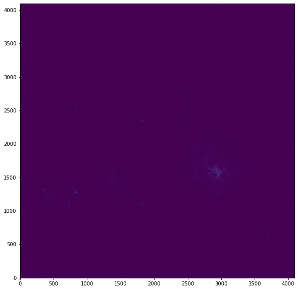
_images/E-1-introduccion_imagenes_astronomicas_43_1.png

Es típico en imágenes astronómica que si representamos de manera líneal la luminosidad de los píxeles la imagen sea muy oscura con una pequeñas manchas de luz en los sitios donde hay objetos muy brillantes. Para mejorar un poco el aspecto podemos procesar los datos de la imagen haciéndoles una transformación logarítmica np.log(data_imagen):

[22]:

plt.figure(figsize=(10,10))
plt.imshow(np.log(data_imagen), origin='lower')

[22]:

<matplotlib.image.AxesImage at 0x7f7f760710a0>

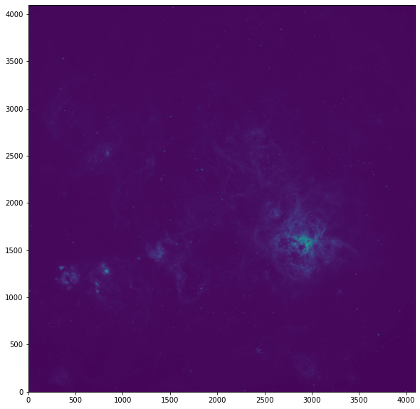
_images/E-1-introduccion_imagenes_astronomicas_45_1.png

Ya somos capaces de distinguir más detalles en nuestra imagen. Hay que resaltar que todavía NO hemos modificado nuestra imagen. Simplemente estamos cambiando la manera de representar visualmente nuestra imagen. Otra posibilidad para ver «mejor» los detalles de la imagen es hacer un estirado del histograma situando el mínimo y máximo en la escala de colores de matplotlib:

[23]:

plt.figure(figsize=(10,10))
plt.imshow(data_imagen, vmin=1000, vmax=2000, origin='lower')
plt.xlabel('píxeles')
plt.ylabel('píxeles')

[23]:

Text(0, 0.5, 'píxeles')

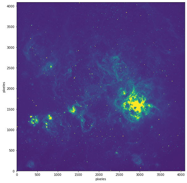
_images/E-1-introduccion_imagenes_astronomicas_47_1.png

Dicho estiramiento del histograma lo podemos hacer no solo especificando valores absolutos, sino obteniendo valores para el mínimo y máximo de la propia imagen. En el siguiente ejemplo estiramos la visualización de la imagen entre el valor minimo de cualquier pixel de la imagen np.min(data_imagen) y un 50% por encima del valor promedio np.mean(data_imagen)*1.5:

[24]:

plt.figure(figsize=(10,10))
plt.imshow(data_imagen, vmin=np.min(data_imagen), vmax=np.mean(data_imagen)*1.5, origin='lower')
plt.xlabel('píxeles')
plt.ylabel('píxeles')

[24]:

Text(0, 0.5, 'píxeles')

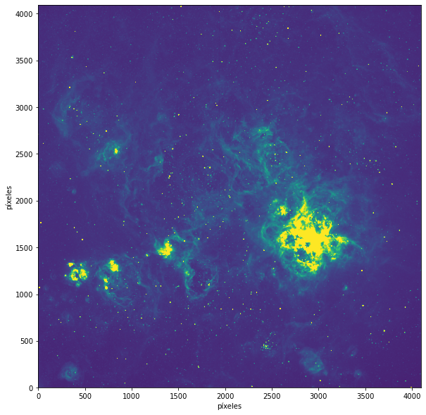
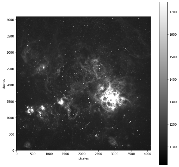
_images/E-1-introduccion_imagenes_astronomicas_49_1.png

Por último nos habremos percatado que matplotlib usa una paleta de colores por defecto entre el azul oscuro y el amarillo (llamada viridis) cuando realmente la imagen que estamos tratando es en tonos de gris. Podemos cambiar la paleta de colores que debe usar e incluso que represente una leyenda al lado de la imagen para tener una idea más clara de los valores que se están representando:

[25]:

plt.figure(figsize=(10,10))
plt.imshow(data_imagen, vmin=np.min(data_imagen), vmax=np.mean(data_imagen)*1.5, cmap="gray", origin='lower')
plt.colorbar()   # Añade la leyenda de la barra de color
plt.xlabel('píxeles')
plt.ylabel('píxeles')

[25]:

Text(0, 0.5, 'píxeles')

_images/E-1-introduccion_imagenes_astronomicas_51_1.png

¿Cómo abrir varios `FITS` a la vez?¶

Lo primero que tenemos que saber es que nuestras imágenes se van a almacenar en una lista. Podemos hacerlo de varias formas: - Abrimos las imágenes como hdul y las vamos incorporando a la lista conheader ydata. - Abrimos las imágenes comohdul pero solo asignamos a la lista los datos. Con esto nos ahorraremos ponerhdul[0].data cada vez que vayamos a operar con las imágenes.

Creamos una lista con la ruta de todas las imágenes¶

Tenemos dos formas de hacerlo: - Mediante la biblioteca Path - Mediante la biblioteca glob

[26]:

from pathlib import Path

nombreImagenes = []

directorio = Path('imagenes/calibracionImagenes/ha/')

for imagenes in directorio.iterdir():  # Iteramos pora todos los ficheros (y directorios) de un directorio

    nombreArchivo = str(imagenes)
    if nombreArchivo.endswith(".fits") or nombreArchivo.endswith(".fit") or nombreArchivo.endswith(".fts"):
        nombreImagenes.append(nombreArchivo)

[27]:

import glob
directorio = 'imagenes/calibracionImagenes/ha/*.fit'
fileList = sorted(glob.glob(directorio)) #glob genera la lista y sorted los ordena

[28]:

nombreImagenes, fileList

[28]:

(['imagenes/calibracionImagenes/ha/NGC2070-20200208@031223-300S-H-alpha.fit',
  'imagenes/calibracionImagenes/ha/NGC2070-20200208@031915-300S-H-alpha.fit',
  'imagenes/calibracionImagenes/ha/NGC2070-20200208@033255-300S-H-alpha.fit',
  'imagenes/calibracionImagenes/ha/NGC2070-20200208@032604-300S-H-alpha.fit',
  'imagenes/calibracionImagenes/ha/NGC2070-20200208@030339-300S-H-alpha.fit',
  'imagenes/calibracionImagenes/ha/NGC2070-20200208@034446-300S-H-alpha.fit'],
 ['imagenes/calibracionImagenes/ha/NGC2070-20200208@030339-300S-H-alpha.fit',
  'imagenes/calibracionImagenes/ha/NGC2070-20200208@031223-300S-H-alpha.fit',
  'imagenes/calibracionImagenes/ha/NGC2070-20200208@031915-300S-H-alpha.fit',
  'imagenes/calibracionImagenes/ha/NGC2070-20200208@032604-300S-H-alpha.fit',
  'imagenes/calibracionImagenes/ha/NGC2070-20200208@033255-300S-H-alpha.fit',
  'imagenes/calibracionImagenes/ha/NGC2070-20200208@034446-300S-H-alpha.fit'])

Lista con `hdul`¶

Este método implica trabajar directamente con los hdul de la imagen y tenemos que estar pendiente de poner [0].dat o [0].header para acceder a los datos de la imagen. Además, podríamos tener problemas a la hora de no cerrar el archivo al final del proceso:

[29]:

from astropy.io import fits

hdul = []

for imagenes in fileList:
    hdul.append(fits.open(imagenes))

[30]:

hdul[0][0].data # hdul[numero de la imagen][tanto los datos como el header del hdul estan en el primario]

[30]:

array([[1159, 1167, 1196, ..., 1078, 1105, 1117],
       [1160, 1178, 1189, ..., 1099, 1093, 1111],
       [1169, 1181, 1154, ..., 1105, 1118, 1099],
       ...,
       [1138, 1132, 1096, ..., 1120, 1118, 1121],
       [1132, 1122, 1118, ..., 1115, 1128, 1137],
       [1124, 1140, 1114, ..., 1102, 1117, 1147]], dtype=uint16)

Lista con los datos de todos los `hdul`¶

[31]:

header = []
data = []

for imagenes in fileList:
    hdul = fits.open(imagenes)
    header.append(hdul[0].header)
    data.append(hdul[0].data)
    hdul.close()

[32]:

header[0]

[32]:

SIMPLE  =                    T
BITPIX  =                   16 /8 unsigned int, 16 & 32 int, -32 & -64 real
NAXIS   =                    2 /number of axes
NAXIS1  =                 4096 /fastest changing axis
NAXIS2  =                 4096 /next to fastest changing axis
BSCALE  =   1.0000000000000000 /physical = BZERO + BSCALE*array_value
BZERO   =   32768.000000000000 /physical = BZERO + BSCALE*array_value
DATE-OBS= '2020-02-08T03:06:15' / [ISO 8601] UTC date/time of exposure start
EXPTIME =   3.00000000000E+002 / [sec] Duration of exposure
EXPOSURE=   3.00000000000E+002 / [sec] Duration of exposure
SET-TEMP=  -30.000000000000000 /CCD temperature setpoint in C
CCD-TEMP=  -30.000000000000000 /CCD temperature at start of exposure in C
XPIXSZ  =   9.0000000000000000 /Pixel Width in microns (after binning)
YPIXSZ  =   9.0000000000000000 /Pixel Height in microns (after binning)
XBINNING=                    1 / Binning level along the X-axis
YBINNING=                    1 / Binning level along the Y-axis
XORGSUBF=                    0 /Subframe X position in binned pixels
YORGSUBF=                    0 /Subframe Y position in binned pixels
READOUTM= '1 MHz   ' /          Readout mode of image
FILTER  = 'H-alpha '           / Filter name
IMAGETYP= 'Light Frame' /       Type of image
TRAKTIME=   5.0000000000000000 /Exposure time used for autoguiding
FOCALLEN=               1936.1 / Focal length of telescope in mm
APTDIA  =   500.00000000000000 /Aperture diameter of telescope in mm
APTAREA =   178678.08714509010 /Aperture area of telescope in mm^2
SBSTDVER= 'SBFITSEXT Version 1.0' /Version of SBFITSEXT standard in effect
SWCREATE= 'MaxIm DL Version 6.09 160704 03UA3' /Name of software
SWSERIAL= '03UA3-CEEN7-J299Y-94VNY-U13XJ-E0' /Software serial number
SITELAT = '-30 28 15' /         Latitude of the imaging location
SITELONG= '-70 45 54' /         Longitude of the imaging location
JD      =   2458887.6293402780 /Julian Date at start of exposure
OBJECT  = 'NGC2070 '           / Target object name
TELESCOP= 'ACP->Astrooptik'    / Telescope name
INSTRUME= 'FLI     '           / Detector instrument name
OBSERVER= 'Telescope3'         / Observer name
NOTES   = '        '
FLIPSTAT= '        '
CSTRETCH= 'Medium  ' /          Initial display stretch mode
CBLACK  =                 1153 /Initial display black level in ADUs
CWHITE  =                 1809 /Initial display white level in ADUs
PEDESTAL=                    0 /Correction to add for zero-based ADU
SWOWNER = 'Ivan Rubtsov' /      Licensed owner of software
JD-OBS  =      2458887.6293403
HJD-OBS =      2458887.6290039
BJD-OBS =      2458887.6298332
OBJCTAZ =             194.8251
AZIMUTH =             194.8251
OBJCTALT=              47.7458
ALTITUDE=              47.7458
OBJCTHA = '01 56 39.40'
HA      = '01 56 39.40'
PIERSIDE= 'EAST    '
READMODE= '1 MHz   '
AMBTEMP =                   17
HISTORY File was processed by PinPoint 6.1.3 at 2020-02-08T03:11:57
DATE    = '08/02/20'           / [old format] UTC date of exposure start
TIME-OBS= '03:06:15'           / [old format] UTC time of exposure start
UT      = '03:06:15'           / [old format] UTC time of exposure start
TIMESYS = 'UTC     '           / Default time system
RADECSYS= 'FK5     '           / Equatorial coordinate system
AIRMASS =   1.35694060364E+000 / Airmass (multiple of zenithal airmass)
ST      = '07 34 00.40'        / Local apparent sidereal time of exp. start
LAT-OBS =  -3.04711111111E+001 / [deg +N WGS84] Geodetic latitude
LONG-OBS=  -7.07647222222E+001 / [deg +E WGS84] Geodetic longitude
ALT-OBS =   1.58000000000E+003 / [metres] Altitude above mean sea level
OBSERVAT= 'CHILESCOPE'         / Observatory name
RA      = '05 37 21.00'        / [hms J2000] Target right ascension
OBJCTRA = '05 37 21.00'        / [hms J2000] Target right ascension
DEC     = '-69 19 31.0'        / [dms +N J2000] Target declination
OBJCTDEC= '-69 19 31.0'        / [dms +N J2000] Target declination
HISTORY File was processed by PinPoint 6.1.3 at 2020-02-08T03:12:20
FWHM    =   3.78270782232E+000 / [pixels] Mean Full-Width-Half-Max of image star
ZMAG    =   1.76985452953E+001 / Mag zero point for 1 sec exposure
EQUINOX =               2000.0 / Equatorial coordinates are J2000
EPOCH   =               2000.0 / (incorrect but needed by old programs)
PA      =   8.92717748132E+001 / [deg, 0-360 CCW] Position angle of plate
CTYPE1  = 'RA---TAN'           / X-axis coordinate type
CRVAL1  =   8.43359148996E+001 / X-axis coordinate value
CRPIX1  =   2.04800000000E+003 / X-axis reference pixel
CDELT1  =  -2.66001231144E-004 / [deg/pixel] X-axis plate scale
CROTA1  =  -8.92717748132E+001 / [deg] Roll angle wrt X-axis
CTYPE2  = 'DEC--TAN'           / Y-axis coordinate type
CRVAL2  =  -6.93257259717E+001 / Y-axis coordinate value
CRPIX2  =   2.04800000000E+003 / Y-axis reference pixel
CDELT2  =  -2.65964401525E-004 / [deg/pixel] Y-Axis Plate scale
CROTA2  =  -8.92717748132E+001 / [deg] Roll angle wrt Y-axis
CD1_1   =  -3.38076526016E-006 / Change in RA---TAN along X-Axis
CD1_2   =  -2.65942919570E-004 / Change in RA---TAN along Y-Axis
CD2_1   =   2.65979746215E-004 / Change in DEC--TAN along X-Axis
CD2_2   =  -3.38029717098E-006 / Change in DEC--TAN along Y-Axis
TR1_0   =   2.04799977556E+003 / [private] X-axis distortion coefficients
TR1_1   =   4.09600822918E+003
TR1_2   =  -9.27752874369E-001
TR1_3   =   9.17573349534E-002
TR1_4   =  -7.71299189613E-001
TR1_5   =  -2.34136010643E-001
TR1_6   =  -7.32598138490E+001
TR1_7   =   7.20318152719E-001
TR1_8   =  -7.24302799606E+001
TR1_9   =  -2.13102413908E+000
TR1_10  =   1.02429158182E+000
TR1_11  =  -2.18328671392E+000
TR1_12  =   1.25055870525E+000
TR1_13  =   2.62261766608E+000
TR1_14  =   3.90939746288E+000
TR2_0   =   2.04799999900E+003 / [private] Y-axis distortion coefficients
TR2_1   =   4.27111011392E-003
TR2_2   =   4.09599166348E+003
TR2_3   =   5.38729172019E-001
TR2_4   =   8.86546806393E-001
TR2_5   =  -1.39307809623E+000
TR2_6   =   1.60951857270E+000
TR2_7   =  -7.04696501405E+001
TR2_8   =  -8.76500526243E-001
TR2_9   =  -7.11088676599E+001
TR2_10  =  -3.52621540448E+000
TR2_11  =  -1.34522966608E+000
TR2_12  =  -8.54364594815E-001
TR2_13  =  -3.65722689398E+000
TR2_14  =   4.72692785031E+000
HISTORY WCS added by PinPoint 6.1.3 at 2020-02-08T03:12:21
HISTORY   Matched 209 stars from the Gray GSC-ACT Catalog
HISTORY   Average residual was 0.29 arc-seconds
PLTSOLVD=                    T / Plate has been solved by PinPoint

[33]:

data[0]

[33]:

array([[1159, 1167, 1196, ..., 1078, 1105, 1117],
       [1160, 1178, 1189, ..., 1099, 1093, 1111],
       [1169, 1181, 1154, ..., 1105, 1118, 1099],
       ...,
       [1138, 1132, 1096, ..., 1120, 1118, 1121],
       [1132, 1122, 1118, ..., 1115, 1128, 1137],
       [1124, 1140, 1114, ..., 1102, 1117, 1147]], dtype=uint16)

Guardando `fits`¶

Para guardar nuestras imágenes usaremos el método .writeto(), pero previamente si hemos dividido el hdul en dos listas con el header y data tendremos que juntarlos en un nuevo hdul. Para ello crearemos un objeto para introducir los datos en un nuevo hdul.

[34]:

hdul = fits.PrimaryHDU(data=data[0], header=header[0])

Necesito un directorio para guardar mis nuevas imágenes si no lo quiero guardar en el directorio donde se encontraba la original. Para ello uso mkdir y me creo un directorio nuevo.

[35]:

import os
directorioSalida = 'salidas/'
try:
    os.mkdir(directorioSalida)
except:
    print(f"El directorio {directorioSalida} ya existe")

El directorio salidas/ ya existe

Por último guardo mi archivo fits con el método .writeto()

[36]:

hdul.writeto(f"{directorioSalida}prueba.fit", overwrite=True)

Si quiero hacerlo con varias imágenes podemos iterar:

[37]:

for i in range(len(fileList)):
    hdul = fits.PrimaryHDU(data=data[i], header=header[i])
    hdul.writeto(f"{directorioSalida}prueba_{i}.fit", overwrite=True)

E: Introducción al trabajo con imágenes astronómicas (FITS)¶

Instalar e importar la biblioteca astropy¶

La cabecera de un fichero FITS¶

Los datos de la imagen FITS¶

Graficando imágenes FITS¶

¿Cómo abrir varios FITS a la vez?¶